Improving Legacy Models Using AlphaFold
(NOTE: Most links on this page will only work correctly when the page is loaded in ChimeraX’s help viewer. You will also need to be connected to the Internet. Please close ISOLDE and any open models before starting this tutorial.)
(The instructions in the tutorial below assume you are using a wired mouse with a scroll wheel doubling as the middle mouse button. While everything should also work well on touchpads in Windows and Linux, support for Apple’s multi-touch touchpad is a work in progress. Known issues with the latter are that clipping planes will not update when zooming, and recontouring of maps is not possible.)
Tutorial: Quickly improving 2rd0 with AlphaFold reference restraints
NOTE: This tutorial assumes that you are already familiar with the basic operation of ISOLDE. If this is your first time using it, it is highly recommended that you first work through at least the Introduction to crystallographic model rebuilding in ISOLDE tutorial before starting this one.
It is no big secret that models built into lower-resolution datasets have historically been fraught with errors, but it can often be surprising to the uninitiated just how big these errors can get. In the introductory tutorial we looked at rebuilding a small 3.0 angstrom model, 3io0, in ISOLDE using only the information available to us from the experimental data. While that case was fairly straightforward, for larger structures, lower-resolution and/or poorer-quality starting models this approach still becomes quite time-consuming and occasionally frustrating. Luckily, with the advent of AlphaFold and its high-quality models of most well-structured regions of proteins, we now have a much better way to quickly and automatically fix most of the problems in legacy models, reducing the interactive component to the (typically few) sites where the AlphaFold model disagrees with the data, and/or the reference restraints need a little help steering the experimental model to the new conformation.
As our example, we’re going to take a look at 2rd0, a 3.05 angstrom structure of the human p110alpha/p85alpha complex. Published back in 2007 as the first structure of p110alpha (aka PI3Kalpha), given the resolution and state of the art at the time it was inevitable that it would contain some errors. Indeed, like most structures of similar resolution and time period its “headline” validation statistics look quite poor by modern standards:
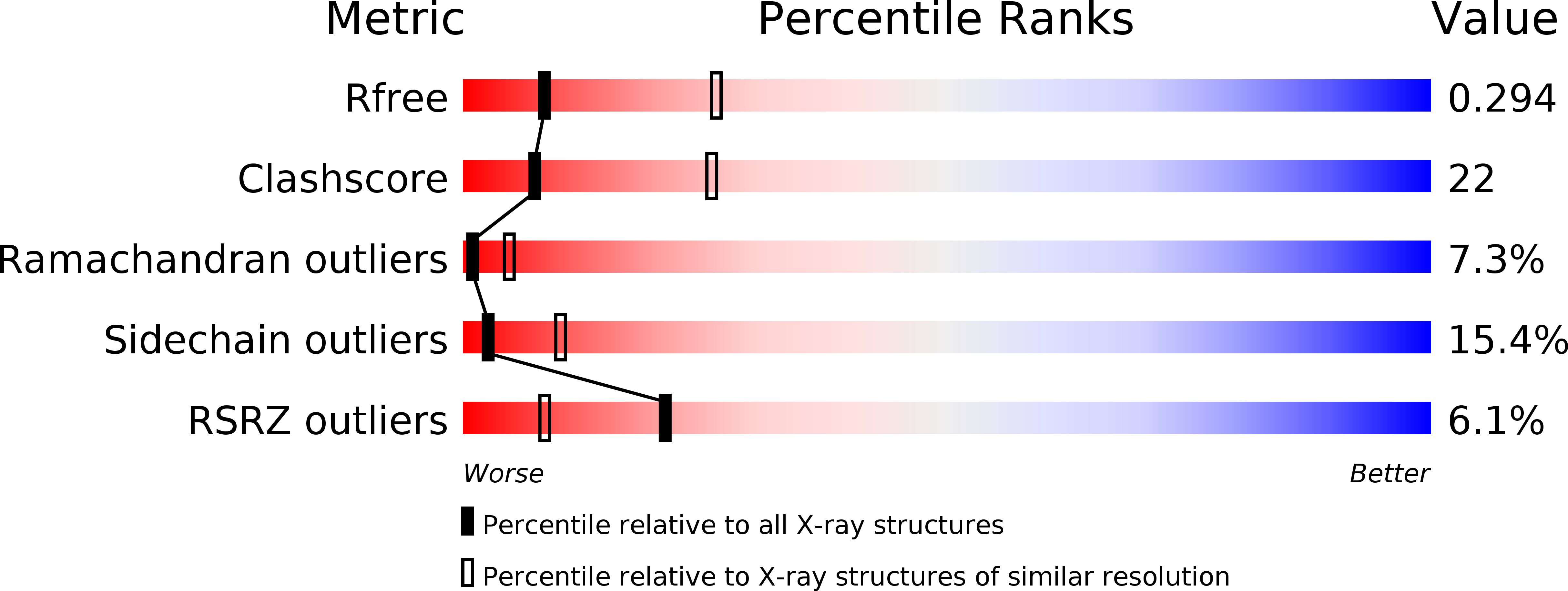
Let’s just take a moment to appreciate the scale of what these values mean. 2rd0 contains 9365 atoms in 1136 amino acid residues. A clashscore of 22 indicates 22/1000, or 206 atoms, are clashing - that is, overlapping in a non-physical way with at least one other atom (in a well-refined structure this should be almost zero). Eighty-two residues are in disallowed Ramachandran space (i.e. their backbones are severely strained) - for a structure this size we’d expect to see 0-2 such cases. It’s not shown in the graphic above, but a further 159 residues (14%) are in the “Allowed” region of the Ramachandran plot where about 2% are actually expected to sit - so in total, that’s at least about 220 residues in need of fixing according to Ramachandran statistics. Finally, 15.4% of sidechains (161 residues) are in non-rotameric conformations - we expect no more than 1-2%.
The point of the above is that there is a lot to be fixed here. While it’s certainly possible to get there in ISOLDE in the absence of any external information, optimistically it would take at least a full working day - and likely quite a bit more. So, let’s explore how we can get there much more quickly.
First, go ahead and open the model and its structure factors. To make the maps a little smoother, we’re going to oversample at a rate of two times the Nyquist frequency rather than the default 1.5.
open 2rd0 structurefactors true oversampling 2
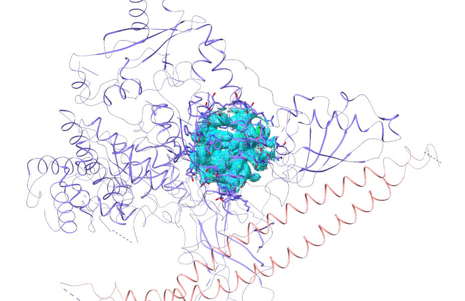
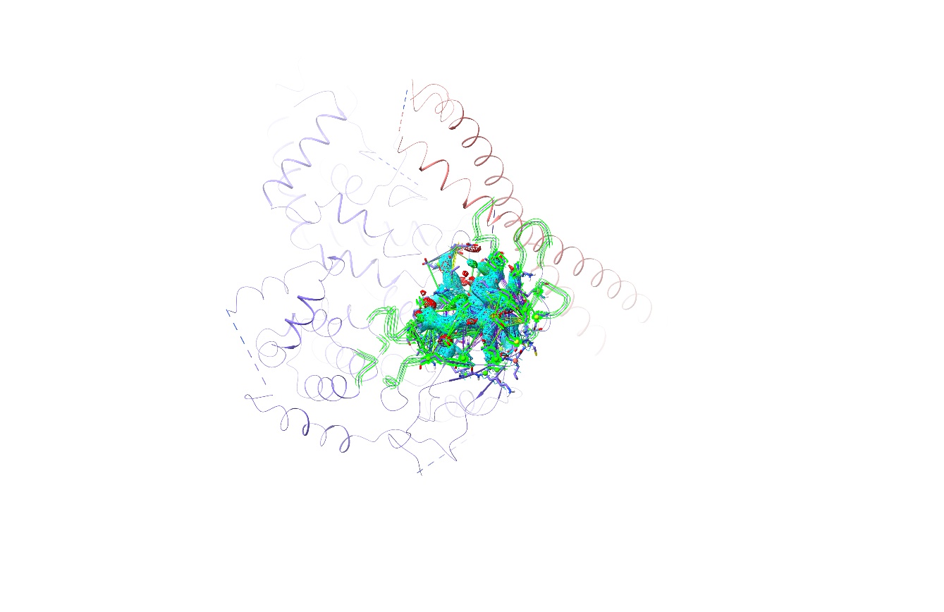
That should give you an initial view looking something like this:
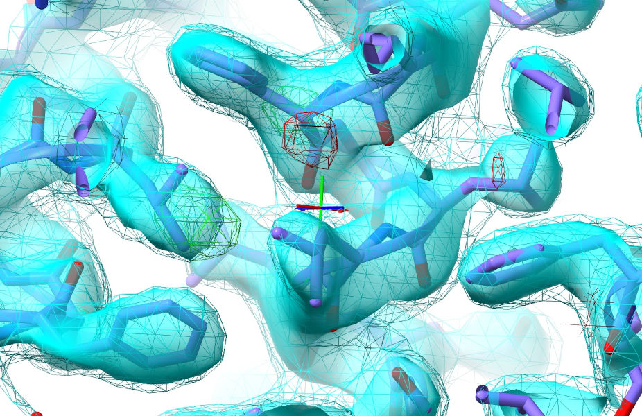
Zoom in (scroll wheel) and adjust the map contours to your liking (ctrl-scroll to select the map to adjust, alt-scroll to actually adjust it. Sigma values will be shown on the status bar at lower left). I’d suggest setting the sharpened map (transparent cyan) to about 2 sigma and the unsharpened one (cyan wireframe) to 1 sigma. Leave the difference map (red/green wireframe) at the default +/-3 sigma. In the well-resolved core that should look roughly like this:
Remember, you can re-adjust contours whenever you need to.
Now, go ahead and start ISOLDE:
... and add hydrogens:
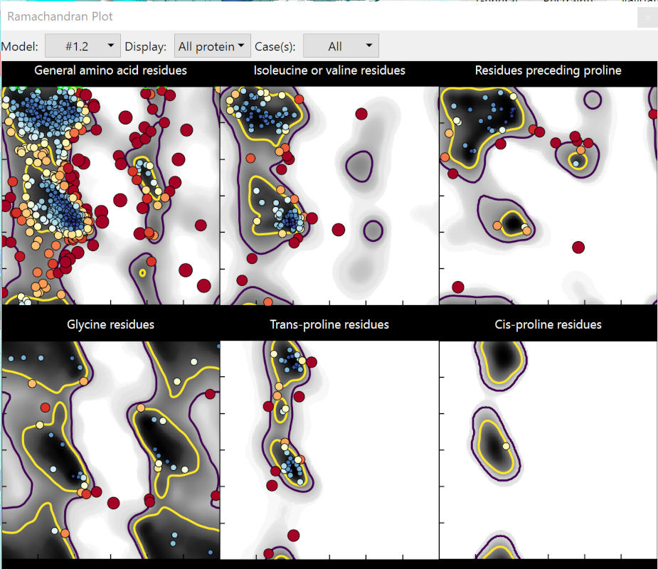
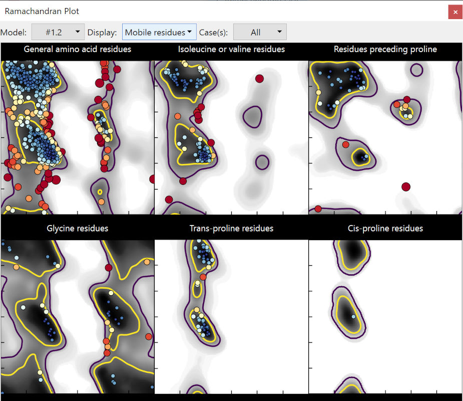
Before we get started properly, take a quick browse through the Ramachandran plots (on the Validate tab). Click on a few outliers to see them in context, and try to picture what needs to be done to correct them.
Now, have a look at what happens if we start a simulation without any reference restraints:
After things start moving, take another look at the Ramachandran plots:
Some clear improvements there. In my session, it’s down to 40 outliers and 89 allowed (from 82/159) - and rotamer outliers are down to 34 (from 161). But there’s still a lot to be done, and of course just because something is no longer an outlier doesn’t mean it’s necessarily correct - it’s always important to see for yourself against the actual experimental map.
Also take a look at the R-factors (on the status bar at bottom right of the ChimeraX window). In my session this simulation increased them slightly from Rwork/Rfree of 0.308/0.352 to 0.317/0.354 (your numbers will almost certainly differ a bit - don’t worry, that’s normal). That’s pretty typical of what happens in ISOLDE for models like this: while regions that were almost right tend to fall into place (and thus improve R-factors), sites that were very wrong and over-fitted will be pushed out of density to resolve energetically unfavourable states (driving the R-factors up, but generally making the problems easier to diagnose and fix).
Anyway, let’s throw out what we just did and revert to the initial state of the model. Hit the big red stop button, or equivalently:
isolde sim stop discardTo start
Now, let’s go ahead and fetch the AlphaFold models for our two chains. (Note: this is only possible for proteins from organisms currently covered by the AlphaFold database - you can see the list of organisms here ):
The optional “trim” argument tells ChimeraX whether or not to automatically trim the predicted models to include only those residues present in the experimental construct according to the sequences stored in the mmCIF file. In order for confidence-based weighting of reference distance restraints to work correctly, this must be set to false. Your display should now look like this:
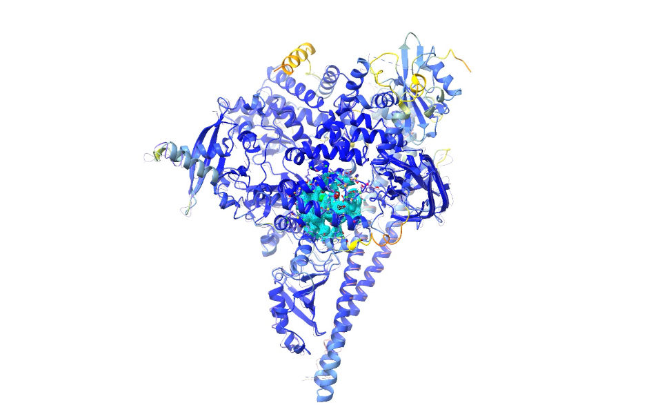
The AlphaFold model is displayed as a ribbon and coloured according to its confidence in its prediction (the predicted local distance difference test, or pLDDT score) for each individual residue (orange = least confident, dark blue = most confident). (IMPORTANT NOTE: residues with pLDDT scores less than about 50 are generally junk and their coordinates should not be interpreted in any way. Nevertheless, it may on occasion be useful to keep them present to start with, to act as raw material for the fitting process. Once the model is fitted it is best to inspect and cull these on a case-by-case basis.)
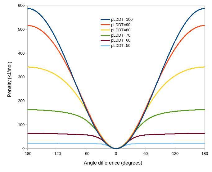
AlphaFold actually provides two different measures of confidence in its predictions, each of which is really useful in its own way. The pLDDT score, a measure of confidence in the conformation and immediate local environment of a residue, is a fairly natural measure to use to adjust the weights of torsion-space reference model restraints. This is achieved with the argument “adjustForConfidence true” of the “isolde restrain torsions” command. The overall effect of the adjustment scheme is shown below - qualitatively speaking, reducing pLDDT will lead to both weaker and “fuzzier” restraints on the matching residue. Residues for which the reference model pLDDT values are less than 50 will not be restrained.
So let’s go ahead and apply these. You can do this chain-by-chain with the Reference Models widget on ISOLDE’s Restraints tab:
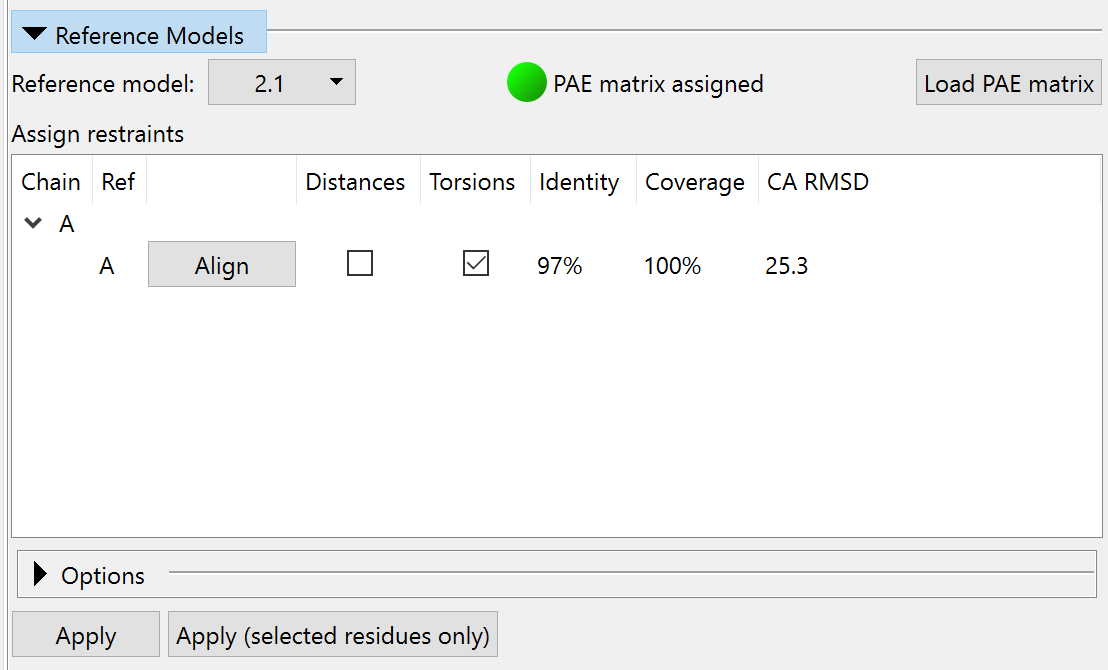
... or using the commands:
isolde restrain torsions #1/A template #2/A adjustForConfidence true
isolde restrain torsions #1/B template #2/B adjustForConfidence true
Let’s take a quick look at the effect of this. First, let’s show all atoms and hide the cartoon for the reference model:
... and zoom in on Leucine 687 of chain A:
The two leucine residues here are good examples of the types of subtle errors that often creep in to low resolution models. Both of them are modelled backwards (rotated ~180 degrees around the outermost chi dihedral) - a severely outlying, strained geometry, but one that appears to fit low-resolution density like this almost as well as the correct state. AlphaFold appears to have gotten it right in both cases, and from the colour we can see it’s very confident about its predictions - this will lead to very strong and wide-ranging restraints here.
Now, let’s move on to distance restraints. Here we have two new arguments added to the “isolde restrain distance” commands. The first, “adjustForConfidence true” is analogous to the torsion restraint case, except that instead of pLDDT it uses the predicted aligned error (PAE) matrix for the prediction to adjust each restraint.
The PAE matrix encodes the confidence AlphaFold has in the distance between every single residue pair in the model (technically, each point [i,j] is the expected error in the position of residue i if the predicted and true structures were aligned on residue j). This is what it looks like for chain A:
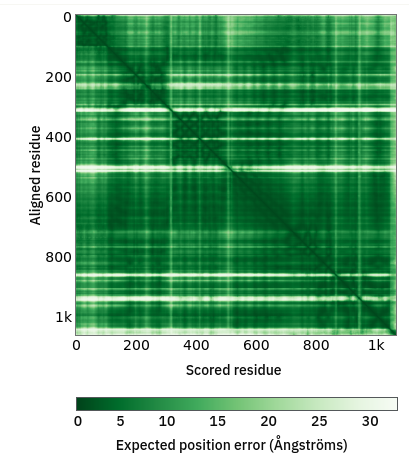
... well, that’s how it’s displayed on the website, anyway. But note the color scale - I’m sure you’ll agree that distances with estimated errors of 30 angstroms aren’t particularly useful for restraint purposes! In fact, ISOLDE only restrains distances for residue pairs with a mutual PAE of 4 angstroms or better. Let’s see what that matrix looks like rescaled to that range:
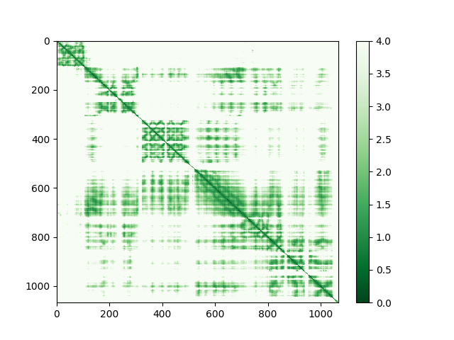
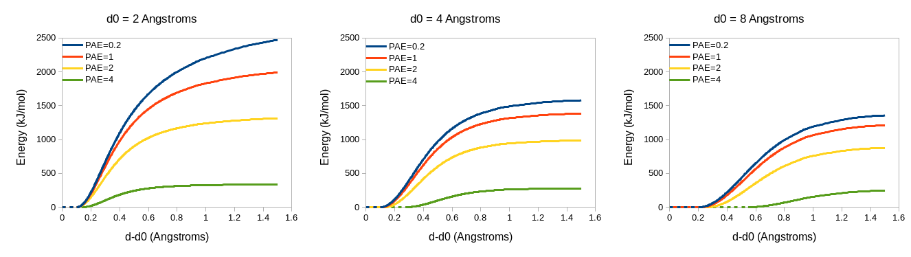
Distance restraints will only be applied on a given pair of atoms if their reference positions are less than 8 Angstroms apart and the PAE between their parent residues is less than or equal to 4 angstroms (i.e. where they correspond to a green dot on the above plot). For residues meeting those criteria, representative plots of the restraint potentials are shown below.
The second new option for the “isolde restrain distances” command is “useCoordinateAlignment false”. This affects how ISOLDE compares the reference and working models in order to assign distance restraints. The default is to do it by a series of rigid-body alignments: find the largest piece that aligns well, assign restraints to those residues; find the next largest piece… and repeat until there is nothing left to align. That generally works well when the reference model is an experimental structure (and particularly when its sequence isn’t identical to the working model), because it avoids generating spurious restraints between domains that have shifted substantially - but it has the drawback that residues that are substantially out of register will typically not be given restraints to their correct interaction partners. With “adjustForConfidence true” the problem of spurious restraints is generally avoided, making the progressive decomposition largely unnecessary. The “useCoordinateAlignment false” command tells ISOLDE to instead assign model/template residue pairs strictly based on sequence alignment only, which makes sure that restraints between confidently-predicted atoms are assigned no matter how badly placed they are in the working model.
Anyway, let’s make it happen. Again, you can do this via the Reference Models widget:

... or via commands:
isolde restrain distances #1/A template #2/A adjustForConfidence true useCoordinateAlignment false
isolde restr dist #1/B templ #2/B adj t useCoord f
Let’s take a look at what that’s done. Hide the AlphaFold models:
... select your working model:
... and expand the map to cover it using the “Mask to selection” button on ISOLDE’s ribbon menu, or:
To get a closer look at an overview of the distance restraints, let’s turn off the map view:
(Note: the exclamation mark in “#!1.1” here tells ChimeraX to change the display setting of only the top-level “container” model for the maps, without changing the display settings of the maps themselves. This is important to make it easy to get back exactly the same view as we had before)
Also, let’s hide all the restraints that are close to satisfied via the Manage/Release Adaptive Restraints widget, or:
isolde adjust distances #1 displayThreshold 0.5
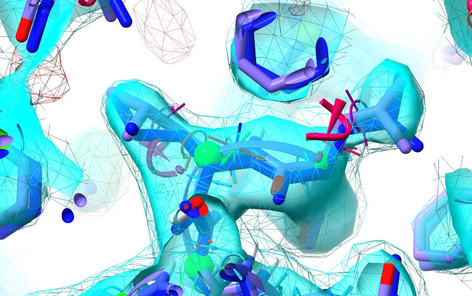
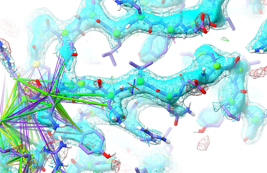
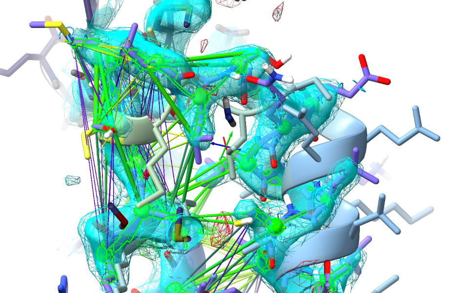
Browse around a bit. You’ll see a lot of purple indicating pairs of atoms that are much further apart than AlphaFold thinks they should be. Let’s focus in on one of these, and bring our maps back:
view #1/A:490-498; show #!1.1 model; clipper spot
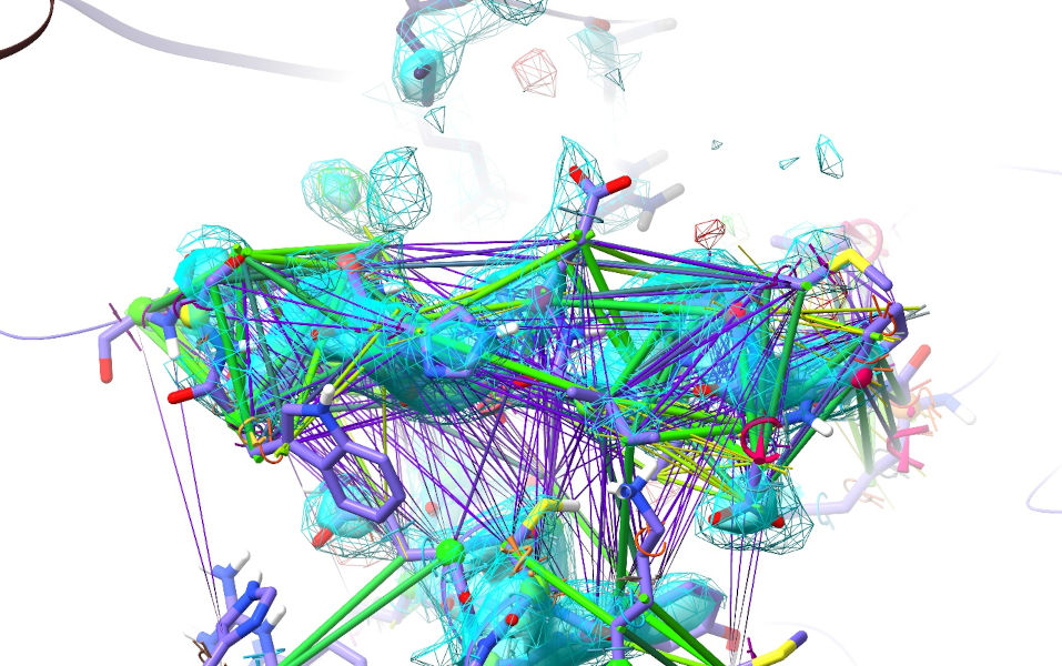
The forest of purple restraints you see here are a telltale giveaway that this helix is probably out of register. Indeed, a close look at the fit to density reveals a lot of red flags: Trp498 has no appreciable density around its sidechain, while there’s a large green difference blob of about the right shape on the other side of the helix; Glu494 is in density much too large for its sidechain (and pointing at Asp578 - not impossible, but something that’s generally only stable at low pH); Met489 is pointing into space while Asp488 protrudes into a hydrophobic cavity.
Now bring up the AlphaFold model for comparision:
Now, I know this image is getting a bit crowded, but a bit of inspection suggests it will solve the above problems. Trp498 goes into that nice difference blob; Glu494 is replaced by His495; Met489 takes the place of Asp488.
... but before we actually fix all that, it’s time to settle the model under the influence of these restraints. First, hide the AlphaFold models for clarity, then start a simulation and wait a while for it to settle, without tugging anything.
If you’re still watching this site, you’ll notice from the still-stretched distance restraints that ISOLDE is unable to fix it automatically.
That’s alright. We’ll get to fixing that in a bit. First, though, let’s take a quick inventory of what ISOLDE has been able to do with the aid of these restraints. Stop the simulation:
... and take another look at the Ramachandran plots:
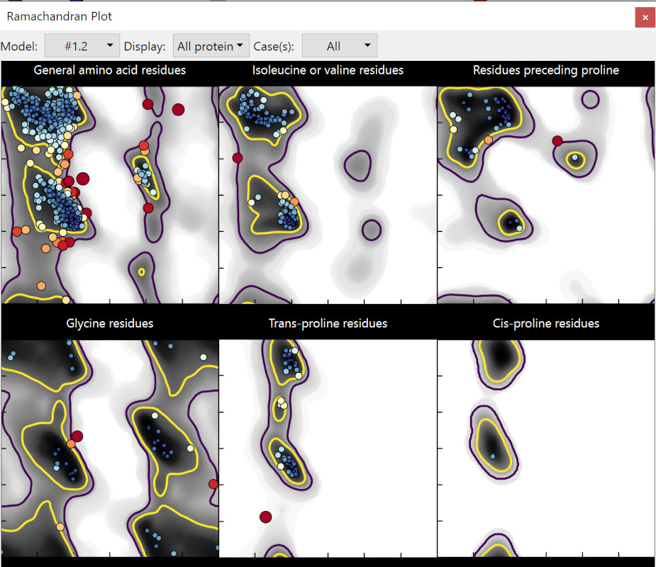
Now we’re getting somewhere! We’re clearly still not done yet, but the statistics are starting to look much more like a real-world protein. We’re down to 14 Ramachandran outliers (1.2%) and 36 allowed (3.2%); rotamer outliers are down to 5. Most importantly, this time the R-factors have tightened substantially (0.326/0.344 vs. the original 0.308/0.352) suggesting we’ve both improved the true fit to the map and reduced a bunch of model bias.
Clearly, there’s still a bunch to be done - but now we’re not going to be shooting in the dark quite as much as we would have been without the help of AlphaFold. The next obvious thing to do is start working through the biggest “problem sites” - mainly those shown up by large clusters of unsatisfied distance restraints. Now, you could do this by simply browsing visually through the structure, but ISOLDE’s problem site aggregator lets you do things a bit more systematically. It looks for all instances of different restraint violations and validation issues and identifies regions where many problems are clustered together - the idea being that such clusters are often the result of a single root cause, so tackling the biggest ones first is likely to give you the fastest overall improvement.
Switch to the “Problem Zones” tab and click the “Update” button at bottom right. You should see something like this (your numbers will almost certainly vary somewhat - don’t worry).
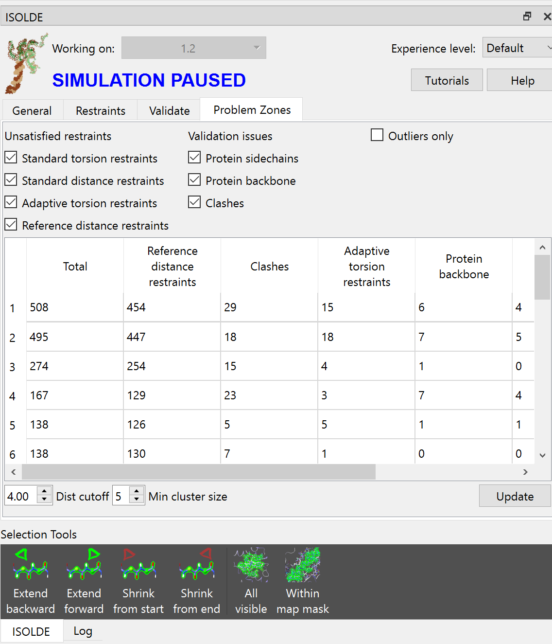
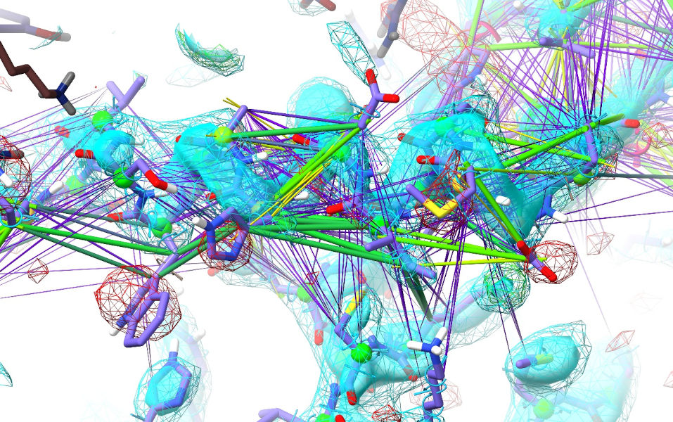
Click on the top row of the table. All atoms associated with problems found in the cluster are selected, and the view is updated to show them:
(NOTE: Depending on how your initial run went, the top cluster may be around either the A355-375 beta-hairpin, or the A488-499 helix. If your top cluster is the helix, choose the second cluster here.)
Click ISOLDE’s play button, or
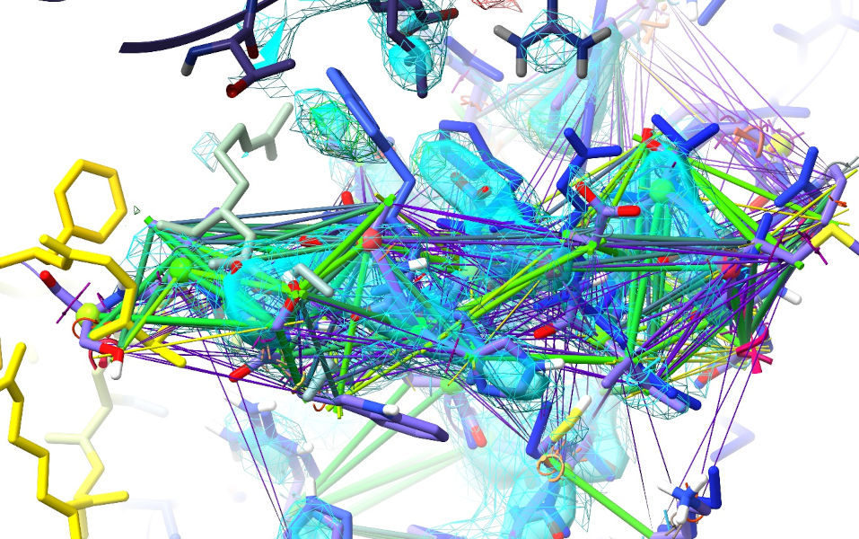
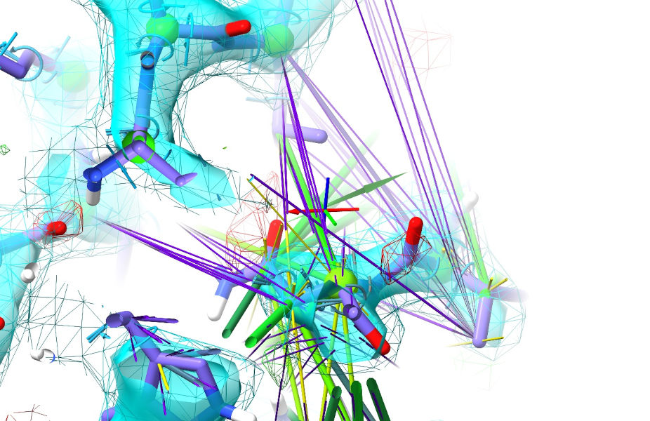
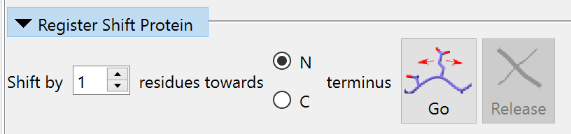
Zoom in, and you should see something like this:
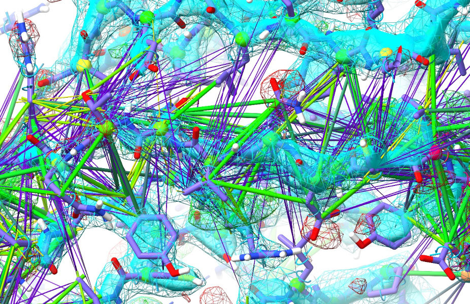
Now, I’ll admit that looks somewhat daunting up-front - but don’t worry, in most cases it just comes down to tugging atoms in the direction of the purple connections, combined with a little common sense and/or help from the reference model. If you spend a little time inspecting without the aid of the AlphaFold model first, I think you’ll agree that 355-362 look solid in their density as do 384-392 - so it’s mainly just that middle 366-378 strand that’s out. See if you can figure out how it’s out - then when you’re ready, show the AlphaFold model to see if it agrees with your assessment.
Spoiler: it’s out by 1, with everything needing to move one residue back towards the N-terminus. This is hard to achieve via simple linear distance restraints like this - atoms that want to go one way around the backbone end up battling atoms that want to go the other - which is why we need to give it a bit of help.
If you find the display too busy, hide the AlphaFold model again. Now, let’s try the simplest (and often fastest) approach - just directly helping out with a bit of right-mouse tugging.
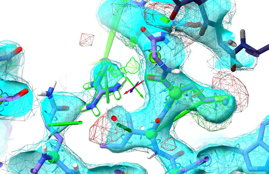
A good place to start might be Asn 372, buried in the hydrophobic core when it wants to be exposed to solvent. Rotate your view so you’re looking along the chain (allowing you to easily tug around the backbone) - if the view gets too busy for you, remember you can shift-scroll to tighten the clipping planes. Grab one of the outermost sidechain atoms, and tug it towards the Val371 sidechain. When tugging, try to steer around the backbone rather than taking the most direct path:
This may take a little playing around - if it’s not cooperating release the atom and try tugging in a slightly different direction. The aim is to “tip” the geometry over the barrier allowing the surrounding restraints to start cooperating - in my case, tugging just this one atom triggered all the N-terminal residues of the strand to fall into place:
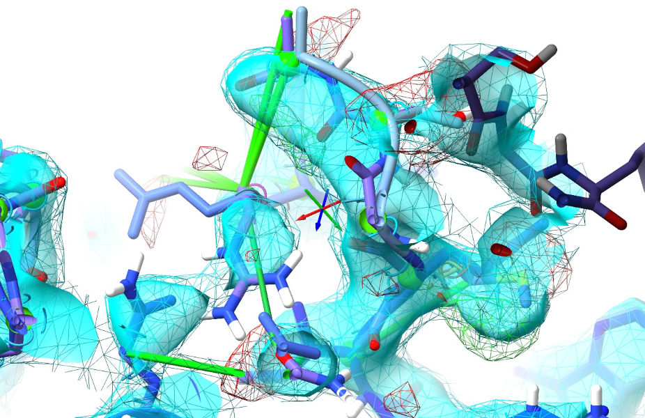
Play around with the rest of the strand - a good next move might be to pull Arg375 outwards. When you’re done, hit the red checkered flag to revert to the original bad geometry and we’ll try using the register shifter instead (this widget on the Restraints tab):
The aim of the register shifter is to provide a somewhat smarter way of applying these large, concerted many-residue shifts. Rather than using distance restraints, it applies a set of moving position restraints to tug the N, C, CA and CB atoms along smooth splines fitted through the positions of their counterparts along the chain. This is a natural way to overcome that problem of distance restraints “fighting” each other. Now, in the past the direction and size of the register shift would have needed to be worked out (or guessed) by careful inspection of fit to density and local interactions; in this case we already know from the AlphaFold model that it’s 1 residue towards the N-terminus. So, select the residues you want to shift:
... dial up the desired shift in the register shifter, then click its button. When it’s done (it should only take a few seconds), click its red ‘X’ to release the position restraints. While Arg375 might still need a little manual help, the rest should just fall into place. Take a little time to clean up the surroundings (hint: Ile351 should really point into the core), and when you’re ready click the green STOP button to stop the simulation and commit the results.
If you’re on the “Problem Zones” tab when you stop the simulation the table will automatically update; otherwise, switch there and click the Update button now. Clicking the top row should now take you to the A488-499 helix. Use what you’ve learned from the previous example to see what you can do with this (Hint: the helix is out by 1-2 residues).
Continue on in this manner, updating the table after each simulation and moving on to the next biggest cluster. After these two, most of the rest get progressively simpler - but you will also start to run into a few sites where the restraints disagree because the AlphaFold model is wrong (or in a “correct”-but-different conformation to what’s in this crystal). A small example is the region around Met772 and Arg777:
Probably not coincidentally, these are right beside a crystallographic interface. Not knowing anything about that, AlphaFold confidently predicts this region with a somewhat-different conformation:
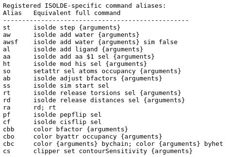
Met772 and Arg777 are predicted with significantly different rotamers, and the 772-777 loop in general doesn’t line up with the density. The best thing to do here is release the local reference restraints and let the density combined with ISOLDE’s force field do the work. Now, you could do this with the “isolde release distances” and “isolde release torsions” commands - but those are a bit long-winded. This is where isolde’s shorthand commands come in really useful. If you enter the command:
... it will enable a series of 2-4 character mini-commands corresponding to common ISOLDE tasks, and print a cheat-sheet to the log:
(HINT: If you go to Favorites/Settings in the ChimeraX menu and then go to the Startup tab, you can make ChimeraX automatically run this command every time it starts)
The ones we’re most interested in here are “rd” (release distance restraints on the selected atoms), “rt” (release torsion restraints on selected residues) and “ra” (release both distance and torsion restraints on the selection). Given that the density here is really strong and at least some of the torsion restraints are wrong alongside the distances, we may as well release both. With a simulation running…
isolde sim start #1/A:770-780,720-730
... select the offending loop:
... and release the restraints:
You’ll want to do a little manual tweaking of the Met772 and Ser774 sidechains (AlphaFold has the latter pointing into symmetry density - swing it around to H-bond to the Lys776 H).
The A217-250 alpha hairpin is another region where the AlphaFold restraints are a bit counterproductive - AlphaFold has the relative disposition of the two helices slightly off compared to the strong local density, and the turn at the top is completely wrong (albeit only predicted with low confidence):
As with the previous case, you’ll want to go ahead and release these restraints. While remodelling this area, you’ll probably also notice a few symmetry clashes. If you want to fix these (and it’s clear that it’s the symmetry-related atoms that are wrong), stop your simulation then double-click on one of the offending symmetry atoms to select and centre the view on its “real” equivalent, allowing you to start a local simulation to fix it before moving on. Don’t be afraid to use a few judicious position restraints if the local density is poor.
Anyway, keep on working your way through until the table is empty. This doesn’t mean that there are no issues left, just that there’s nothing left meeting the definition of a “cluster”. This is the point where, if you were planning on depositing this model to the wwPDB or using it in any downstream application, you’d want to give it a final detailed residue-by-residue inspection to be absolutely certain. (HINT: you can get to the first polymeric residue in your structure with “st first” and continue stepping through by repeating the “st” command) But before doing that, it would be a very good idea to run a refinement at this point to make sure you’re working with the best possible maps. To write input ready for phenix.refine, first navigate to a suitable directory with the command:
cd browse
... then do:
isolde write phenixRefineInput #1 numProcessors 6
(NOTE: due to the way these interactive tutorials are implemented, you will need to type - or copy/paste - these commands into the command line yourself, otherwise the files will be written to the wrong directory.)
This will write a snapshot of your current model (without hydrogens unless you use the optional “includeHydrogens true” argument) along with an MTZ file and a phenix.refine settings file (refine.eff). To run a refinement, navigate to the working directory in a separate operating system terminal window with the Phenix environment activated, and do:
phenix.refine refine.eff.
... then load the results in a fresh ChimeraX session and continue with your final inspection and tweaking. At this resolution, after refinement you should be able to continue on without further use of the AlphaFold restraints.
Here’s what the validation statistics for my model looked like after that refinement step compared to the original deposited structure:
Validation measure |
Original model |
Rebuilt and refined |
|---|---|---|
R-work |
0.291 |
0.238 |
R-free |
0.338 |
0.273 |
Clashscore |
22.64 |
1.50 |
Ramachandran outliers |
7.33% |
0.00% |
Ramachandran allowed |
14.22% |
1.98% |
Ramachandran favoured |
78.44% |
98.02% |
Ramachandran Z-score |
-5.60 |
0.55 |
Rotamer outliers |
17.15% |
0.38% |
C-beta deviations |
1.10% |
0.00% |
Twisted peptides |
0.93% |
0.00 |
Not a bad improvement, I think!