Building Into CryoEM Maps With Your Own AlphaFold Multimer Models
NOTE: Most links on this page will only work correctly when the page is loaded in ChimeraX’s help viewer. Unless the necessary files have been pre-fetched you will also need to be connected to the Internet. Please close any open models before starting this tutorial.
The instructions in the tutorial below assume you are using a wired mouse with a scroll wheel doubling as the middle mouse button. While everything should also work well on touchpads in Windows and Linux, support for Apple’s multi-touch touchpad is a work in progress. Known issues with the latter are that clipping planes will not update when zooming, and recontouring of maps is not possible.
If you wish to leave this tutorial part-way through and return to it later, you can save the state (all open models, maps, restraints etc.) to a ChimeraX session file via the File/Save menu option or with the command:
save tutorial_session.cxs
You can of course also save the working model to PDB or mmCIF - again, via the menu or with your choice of the below commands:
save model.pdb #1
save model.cif #1
To save without hydrogens, instead do:
sel ~H; save {your choice of filename and extension} selectedOnly true
The above commands will save to your current working directory. They are not provided as links here because that would save them to the directory containing this tutorial file, which is probably not what you want.
Tutorial: Fitting a new cryoEM map starting from an AlphaFold multimer prediction
Level: Moderate
This tutorial will write a number of files to your current working directory. To avoid clutter and confusion it is best if you create and change to a fresh directory first.
Click here to choose a directory and populate it with tutorial data
Historically, the typical approach to building an atomic model into a new crystallographic or cryoEM map was “bottom-up”: starting either from nothing or some partial model representing the rigid, conserved core, the chain(s) would be traced through the density by some combination of automated algorigthms and manual building. With the advent of largely-reliable machine learning-based structure predictions heralded by the release of AlphaFold, it is now usually both faster and more reliable to instead take a “top-down” approach, starting from (the) AlphaFold prediction(s) and refitting them into the new experimental map.
For this tutorial, we are going to largely recapitulate 7drt, the 2.2 Angstrom structure of the human Wntless:Wnt3a complex. Published in 2020 and released in 2021, this is the first representative of this complex in the wwPDB and was not included in the training set for AlphaFold2 or the later multimer implementation, making it an excellent test case to explore the strengths and weaknesses of this approach.
Let’s start by taking a look at the original model and map:
open 7drt; open 30827 from emdb; color bychain
... and make it a little more pretty:
volume #2 rmsLevel 8 step 1;color zone #2 near #1; lighting soft
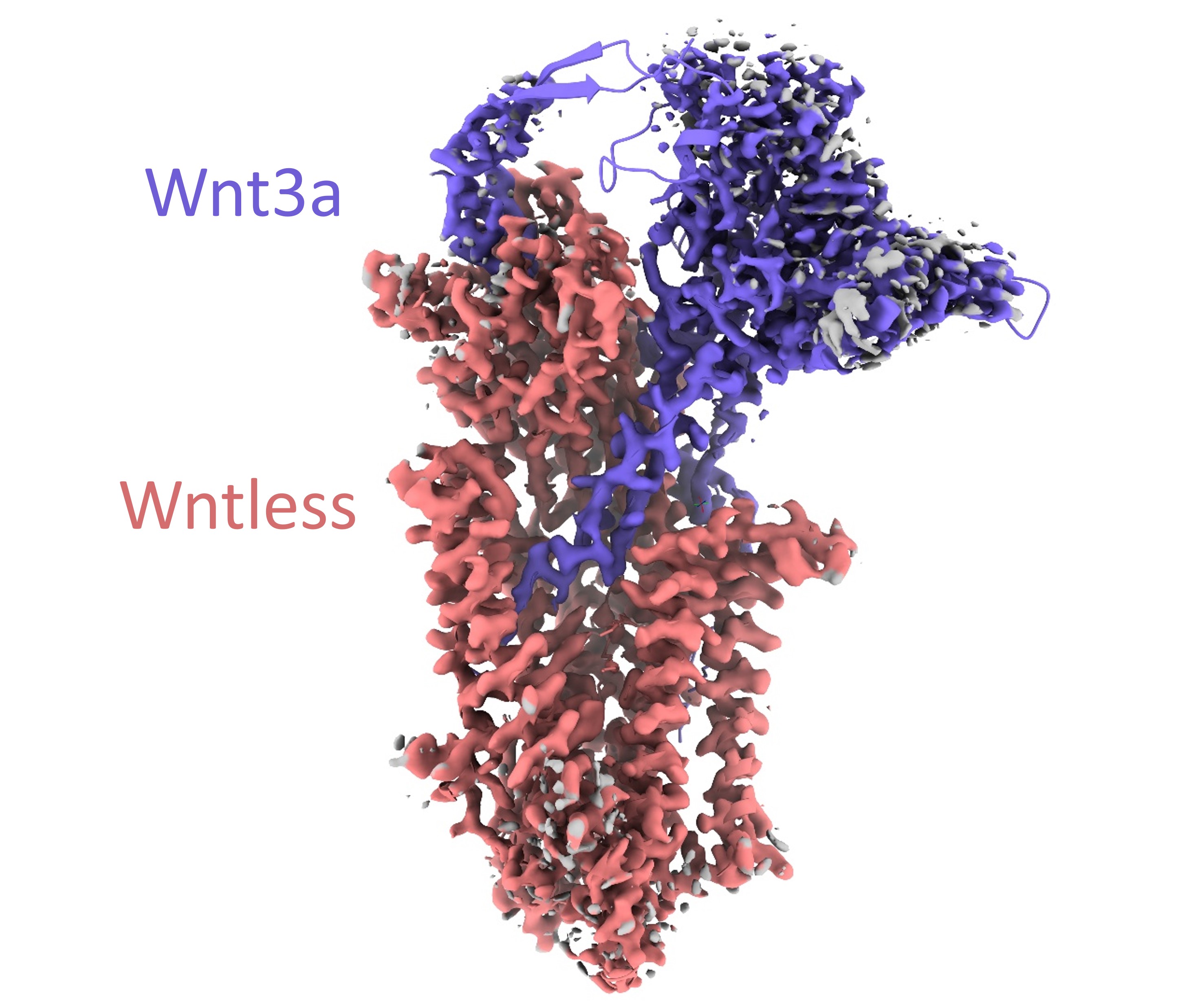
The first thing you might note when looking at this is that, as in many cryoEM reconstructions, that “2.2 Angstrom” resolution is a nominal value relating to the best-resolved parts of the map (in this case the transmembrane domain), and that other regions have significantly lower resolution - revealed as noisy and/or absent density at this contour level. The resolution around the top of the Wnt3a chain is particularly poor - in sites like this we’ll have to rely heavily on prior knowledge.
Preparing the predicted model
Our first step in building into this map based on a predicted model is, of course, to actually generate the model. There are now many tools you can use for this, most of which make use of Google Colab so you don’t need to have an AlphaFold installation on your own computer. Examples include the official DeepMind version, the ColabFold version using a faster multiple sequence alignment implementation, and the ChimeraX version directly launchable from within ChimeraX.
In my experience each of these yields quite similar results, so your choice of which to use is mostly a matter of preference. Except for very small “toy” examples they’re still too slow to run in the context of an interactive tutorial, so here we’ll be working with the stored results from a ColabFold run (which took about 1.5 hours to generate 5 independent predictions of this complex).
Before we get started properly on this, we need to consider a few caveats. While these predictions are often startlingly good, for various reasons they are rarely perfect. The first and most obvious of these reasons is that the prediction only gives one conformation - even if this correctly represents a natural state of the protein, that is not necessarily the same as your state. Other potential issues include:
AlphaFold2 was trained on essentially the entire protein cohort in the wwPDB, with very little filtering for resolution or model quality. As a result, it sometimes makes errors in sidechain geometry similar to those commonly seen in human-generated experimental models.
In places where there is too little information to control things (generally because a site is intrinsically disordered) the local geometry can rapidly degrade into nonsense. It’s important to make sure we discount sites like this.
For multimers like this where there is no pre-existing structure in the training set, it has to rely entirely on sequence coevolution combined with whatever it has learned about what “belongs together” to guide the fold. Importantly, due to the design of the multimer algorithm it only works for complexes where all chains are from the same organism, and does best on tightly-conserved “exclusive” complexes (those with few or no non-interacting paralogs). Don’t expect a sensible result if you try to predict an antibody:antigen complex, for example.
AlphaFold2 knows nothing of ligands or post-translational modifications (or of physics, for that matter). Nevertheless, it will often recapitulate geometry with space for the missing ligands.
Anyway, let’s go ahead and get started. The first link you clicked back at the start created a new directory ‘7drt’ in your working directory with four files in it (two models and two JSON files containing their Predicted Aligned Error (PAE) matrices). A real run of ColabFold typically creates 5 models and returns a few other useful files, but these are omitted here to save space. Anyway, go ahead and open the top-ranked model (“7drt_20b0f_unrelaxed_rank_1_model_4.pdb”) via the ChimeraX File/Open dialog.
Docking into the map
Before doing anything that involves moving your model, it’s best to reduce the lighting effects back to the simple mode - ambient occlusion is beautiful, but expensive to calculate!
At present ChimeraX does not provide an algorithm that will dock a model into a map starting from a random position, so you will need to do the initial work yourself. Of course in this case we could cheat by aligning to the existing experimental structure with
... but the more general solution is to get most of the way with the “Move Model” right mouse mode, then use FitMap to optimise the fit. Go to the “Right Mouse” tab on the ChimeraX ribbon menu and click the “Move model” button (fifth from the right), or use the command:
ui mousemode right “translate selected models”
Then select the AlphaFold model:
and to make things fair, hide the experimental model:
Now, right-click-and-drag will move the model across the screen. Pressing shift while dragging (AFTER clicking and holding the right mouse button) changes this to rotation. Left-click-and-drag rotates the display, and scroll zooms. Use these actions to bring your model approximately into line with the density. Once you think you’re close enough, do:
If the result isn’t to your liking, shift the model a bit and try again. You’ll probably notice quite quickly that it’s impossible to get a satisfactory fit to the transmembrane domain, because the helices are shifted substantially relative to each other. Instead, focus on optimising the fit of the big beta-sandwich domain of Wntless:
You can limit fitMap to only consider this domain with:
Don’t worry that the fit isn’t perfect - after all, that’s what we’re here to fix! But credit where it’s due - considering that when AlphaFold2 was trained there was no experimental structure for this complex (or any homologue) this model is amazingly good. Anyway, if at least part of the model is well-fitted, that makes everything following that much easier.
At this point, it’s finally time to initialise this model for ISOLDE. First, let’s close the experimental model:
If you haven’t already launched ISOLDE, start it now:
Then, click the “Working on:” button at the top left of the ISOLDE window, or alternatively use the command:
A dialog box will appear noting that the model looks like it should have disulfide bonds that aren’t specified in the metadata and asking if you wish to create them. Choose “Yes”.
NOTE: when first prepping a model, ISOLDE temporarily removes it from the ChimeraX session before returning it under the control of a higher-level “manager” with the first available model ID. If you have followed the instructions in this tutorial the structure now becomes model #1.
Before we associate the map with the model and start rebuilding, it would be a good idea to take a quick look at its quality. For clarity, let’s temporarily hide the map:
Now, go to ISOLDE’s “Validate” tab and open the Clashes widget.
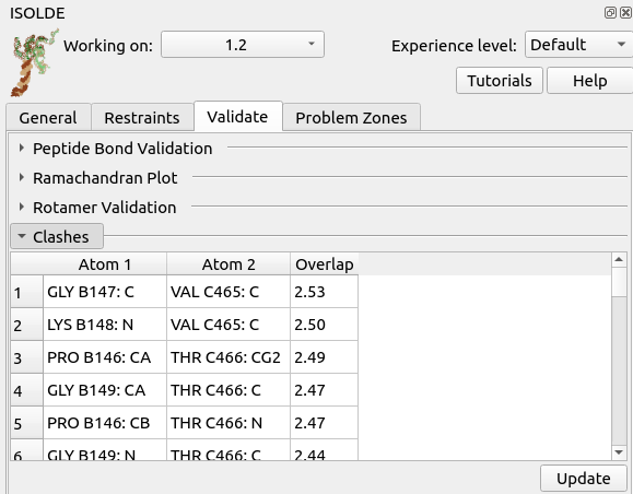
Hmmm - that’s not a good sign. A carbon-carbon overlap of 2.5 Angstroms means the atoms are occupying almost the same position, which could be a real headache to untangle. Click on the top entry in the table to take a closer look.
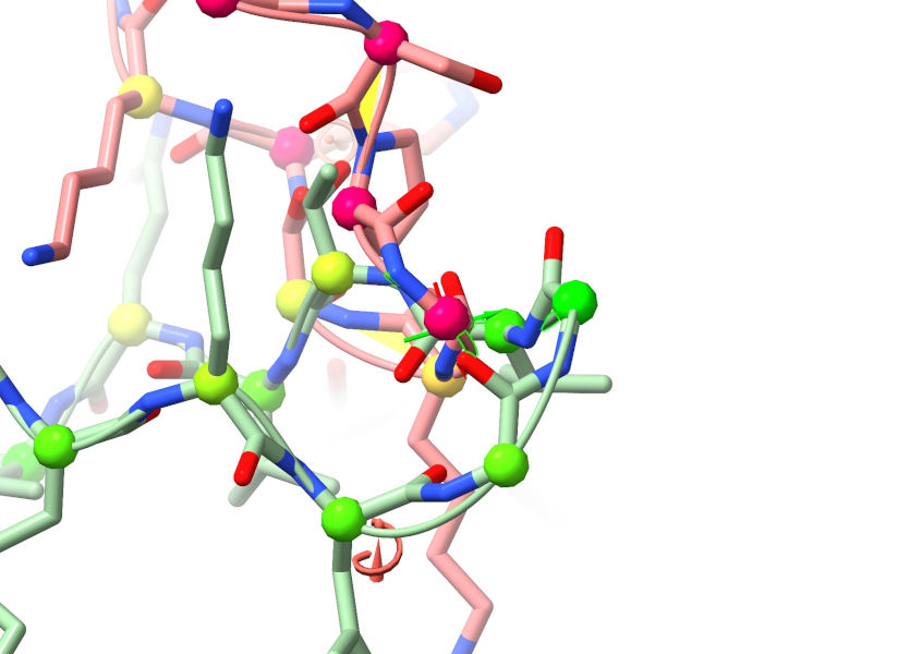
Ugh. That’s not good. This looks like an instance of one of the known deficiencies of AlphaFold: when two stretches (a) are distant in sequence space and (b) have no mutual information controlling their relative positions, in key stages of the algorithm they don’t “know” about each other and can end up overlapping like this.
While a situation like this is reasonably straightforwardly recoverable by temporarily reducing the strength of ISOLDE’s nonbonded potentials (see Dealing with severe clashes), let’s see if we can avoid the issue by using the second model instead. Go ahead and open that (“7drt_20b0f_unrelaxed_rank_2_model_5.pdb”) with the File/Open dialog, and align it to the working model:
You might find it easier to compare if you temporarily hide all atoms:
Indeed, that looks much better. Let’s run with this model:
Click “Update” in the clashes widget, then click on the top entry in the table.
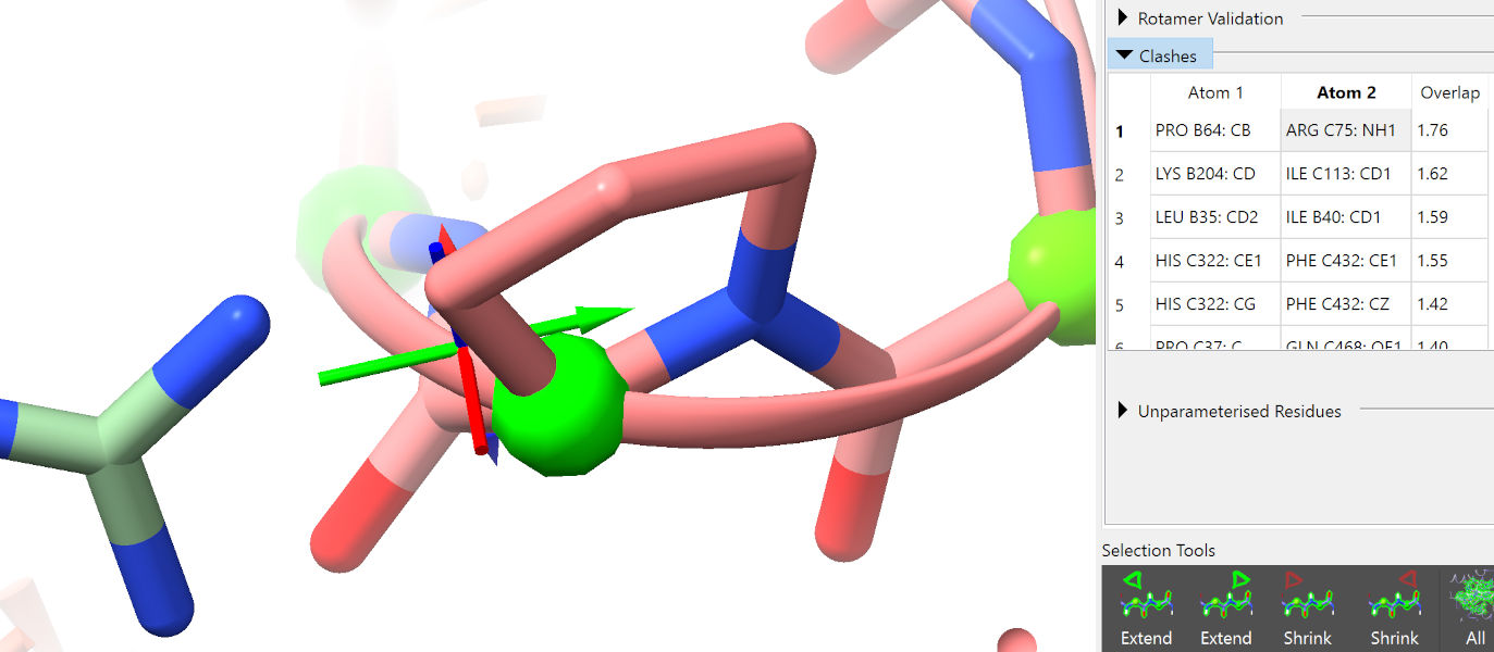
While not ideal, a clash like this (simply requiring the atoms to push apart) is trivial for ISOLDE to deal with, and will not be an issue. Click through the next few entries in the clash table to confirm that they are similar.
While we’re at it, let’s take a look at the other validation tools. Collapse the Clashes widget and bring up the Rotamers widget.
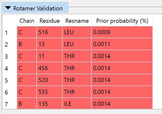
As it stands, the model has 40 sidechains (about 5.2% of rotameric residues) in outlier conformations - much higher than one would expect in a high-resolution experimental model. It is somewhat telling that the majority of these are the same types (LEU, ILE, THR, ASN, HIS) that humans often get wrong in low-resolution maps: small groups whose orientations quickly become ambiguous when relying on density alone for guidance. Many other AlphaFold models are actually much better than this - a possible (but highly speculative) explanation is that at the time of its training, there were very few high-resolution transmembrane models in the wwPDB, causing an extra-strong bias towards these almost-certainly-erroneous conformations in these cases. Whatever the explanation, for now all we can do is take note and move on - once again this emphasizes that while AlphaFold models are good, they are not perfect and certainly can not substitute for experimental structures in most cases.
Anyway, close the Rotamer validation panel. Before we move on, to aid in interpretation of the following validation tools let’s color the model according to AlphaFold’s confidence metric (predicted Local Distance Difference Test, or pLDDT, stored in the B-factor column of the model):
color bfactor #1 palette alphafold
This colours the model red in very low-confidence regions, through orange and yellow to blue for very high-confidence.
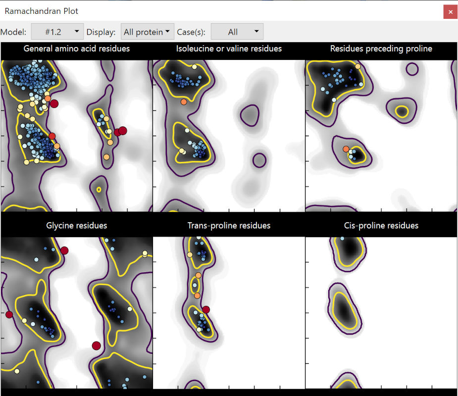
Expand the Ramachandran plot widget, and click the “Launch Ramachandran Plot” button. In the window that pops up, set the “Case” drop-down menu to “all”. Explore a bit, and you’ll notice that many of the most serious problems are clustered in the red tail at the C-terminus of Wntless (chain C… for reasons unclear, ColabFold models always start at chain B):
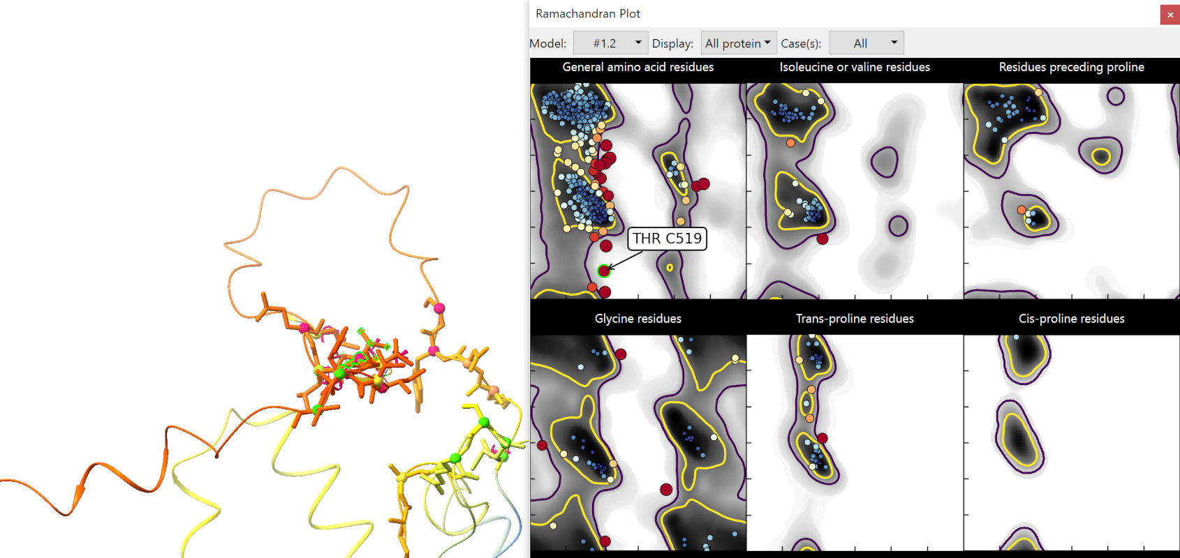
It has been noted by multiple groups now that these very-low-confidence regions in AlphaFold2 models are actually excellent predictors of local disorder. In these regions AlphaFold essentially gives up entirely on trying to impose physical sensibility, beyond keeping adjacent residues bonded to each other. This stretch isn’t going to help us much, so we may as well remove it now:
(HINT: hovering the mouse over any atom will bring up a tooltip identifying it)
The Ramachandran plot looks immediately somewhat better:
Let’s move forward. Close the Ramachandran plot by clicking its window close button or using the command:
ui tool hide “Ramachandran Plot”
Set the model back to the default colour scheme. The full command for this is:
color #1 bychain; color #1 byhet
... but if you first run the command:
... then a bunch of commands commonly used in ISOLDE (including this one) are reduced to simple 2-4 character aliases - a full list will be printed to the log. The equivalent command to the above is simply:
(or simply cbc to colour all open models by chain).
(HINT: to permanently enable this shorthand, go to Favorites/Settings on the ChimeraX menu, choose the Startup tab, and add “isolde shorthand” on a new line in the box titled “Execute these commands at startup”)
Now, let’s show the map:
... and associate it with our working model. You can do this with the “Add map(s) to working model” widget on ISOLDE’s General tab, or with the command:
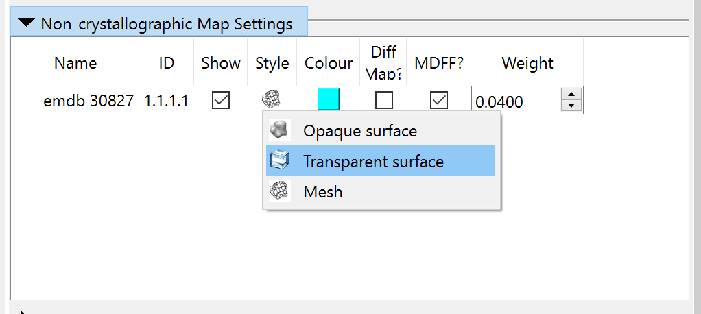
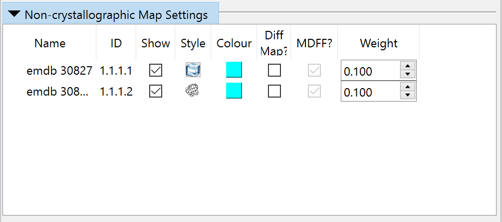
By default the map will appear as wireframe; if (like me) you prefer a transparent surface view you can choose that in the “Non-crystallographic Map Settings” widget:
Before we can actually simulate anything, we need to add hydrogens to the model. May as well do that now:
In our earlier inspections we noted that most of the transmembrane helices are currently well out of step with the map - far enough that if we were to simply try to settle the model into place all we’d end up with is a tangled mess. To allow it to settle sensibly, we’re going to need to reinforce things a bit. That’s where the “Reference Models” widget on the Restraint tab comes in. First, open a second copy of the model to act as a reference.
You might ask why you can’t simply use the existing model as its own reference in this case - and that would be a very valid question. The answer is that we will be using AlphaFold’s Predicted Aligned Error (PAE) matrix to adjust the strength and “fuzziness” of our reference restraints. The PAE matrix is a (n_residues x n_residues) matrix where each position encodes the expected error in placement of one residue when the model is aligned on the other. To avoid a huge amount of potential confusion, the implementation of this expects the reference model to be the original, with no residues added or removed.
Anyway, expand the “Reference Models” panel, and choose model #2 in the “Reference model” drop-down menu.
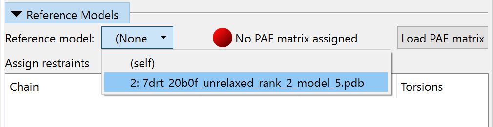
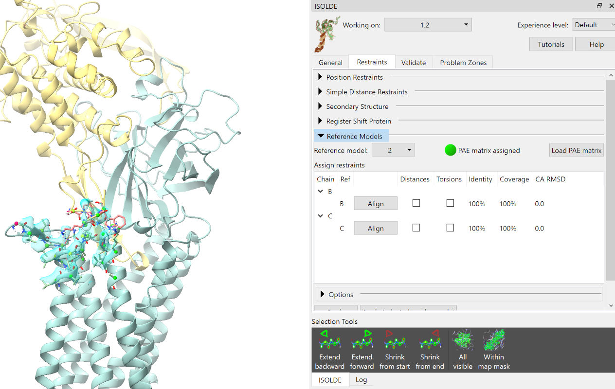
The reference model will automatically be aligned to your working model, and coloured by chain with colours shifted somewhat to differentiate it. To enable weighting of distance restraints by PAE, click the “Load PAE matrix” button and choose the file “7drt_20b0f_unrelaxed_rank_2_model_5_scores.json”. If you have done things correctly, your display should now look something like this:
Check all four checkboxes under “Distances” and “Torsions”. While the parameters of the restraints to be applied may be fine-tuned somewhat on the “Options” panel, here we’ll stick with the defaults (which should look like this, if you can’t resist playing):
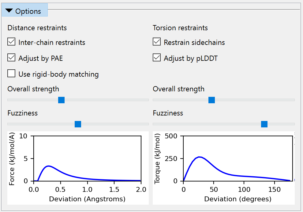
Click the Apply button to assign the restraints. Once this is done you can safely close the reference model… but let’s keep it around for now so we can compare later, and just hide it:
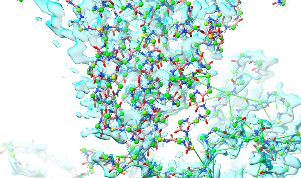
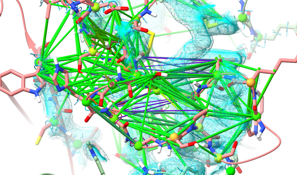
Zoom in on your model and take a look around. You’ll see torsion restraints added to each amino acid phi, psi and chi torsion, and a cobweb network of distance restraints:
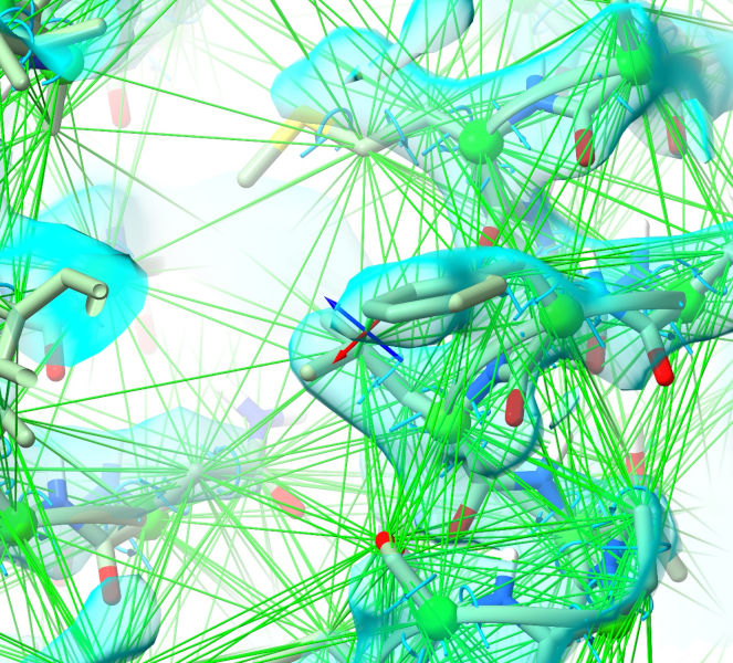
Right now these all look the same because they are (of course) all optimally satisfied - but that will change in a minute or two, since now we’re ready to start a simulation.
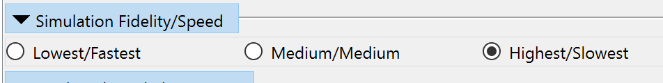
Well, almost. If you’re working with a reasonably high-end Nvidia GPU you’re ready to start now, but if not you should consider switching down to a simpler lower-fidelity simulation mode, which will give you much faster speed at the cost of somewhat poorer handling of electrostatics (largely mitigated in this case by our reference restraints). You can find the widget for this on ISOLDE’s General tab:
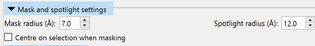
Because we know in advance that some parts of the model will be moving fairly substantially, it wouldn’t hurt to increase the mask radius to, say, 7 Angstroms:
Once you’re happy, select the whole model:
... and either click the “Start simulation” button on ISOLDE’s ribbon menu:
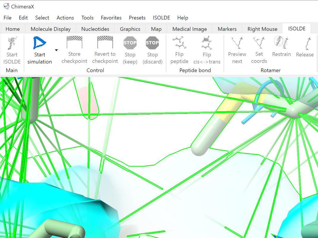
... or use the command:
(equivalent shorthand: ss)
To make interpretation easier at this early “bulk” stage, you might want to reduce the display to just the backbone with:
... or all the way to a C-alpha trace with hide ~@CA
For this tutorial, I’ll take the former option.
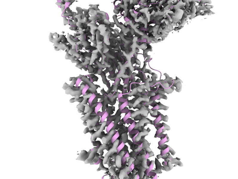
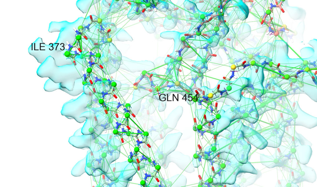
Let things settle for a little while (10-20 seconds on a high-end GPU, longer on lower-end hardware), then pause and have a look around, focusing for now on the transmembrane domain. While most of the transmembrane helices settled into place quite readily, two helices in particular (roughly residues 373-454) started way outside their target density and are unable to settle without help.
To deal with this, first stop the simulation with the green stop button to keep the current coordinates:
... or the equivalent command:
Note that this will reinstate the all-atom view (by design, anything you do to change the atom display during a simulation lasts only for the duration of that simulation).
Now, let’s start a more selective simulation encompassing only this problem region, plus a little padding:
Switch to ISOLDE’s Restraints tab, and expand the “Manage/Release Adaptive Restraints” widget. First, let’s reduce the visual clutter a little by adjusting the distance restraints’ display threshold to hide satisfied restraints:
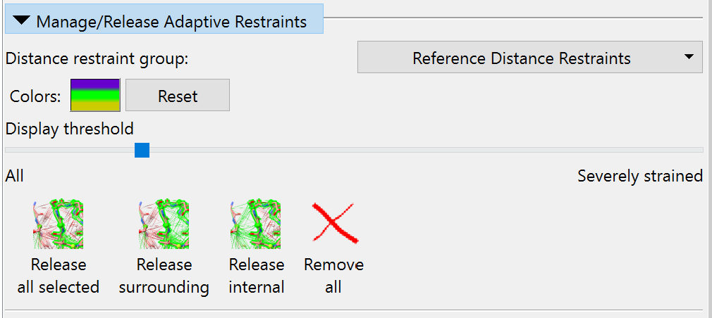
Now, it’s clear from looking at the model and density that while the local restraints maintaing these helices are quite sensible, the restraints between helices are not doing anything except hold the atoms away from the map. So, let’s selectively release those. Select one of the helices by first ctrl-clicking on an atom, then pressing the keyboard up arrow twice to expand the selection to the whole secondary structure element. Then click the button labelled “Release surrounding” or use the shorthand command:
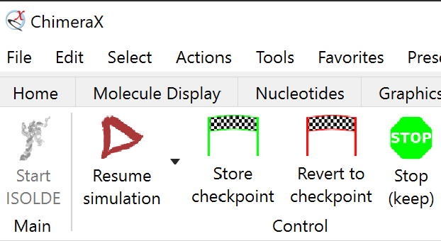
Do the same for the second helix. If the simulation is paused, resume it.
In my case this allowed the 373-411 helix to settle into place on its own (barring a few clearly-wrong rotamers, which we’ll get to in a bit), but the 420-455 helix still needed a little help. At its N-terminus a little mouse tugging was all that was needed to point it in the right direction, but the C-terminal end was more problematic. Firstly, the restraints to the surroundings of the following beta-hairpin:
... which helps things a bit - but there’s still one more barrier. AlphaFold has chosen incorrect rotamers for phenylalanines 449 and 473, and they are currently bashing against each other.
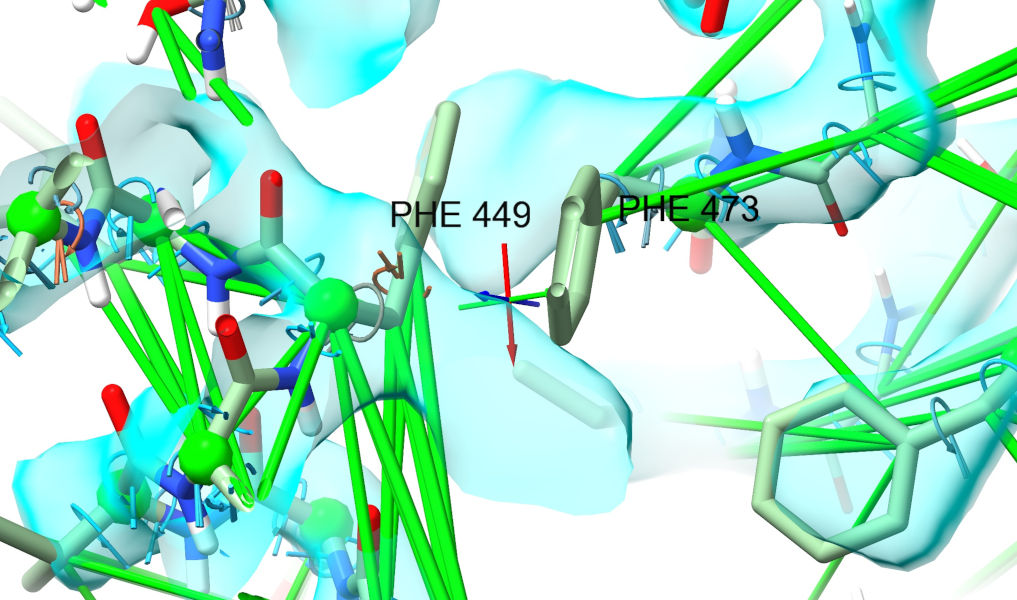
To fix that, we’ll have to release their restraints and adjust. Select both residues - either ctrl-click one, ctrl-shift-click the other and then press up, or use the command:
Then either click both “Release all selected” buttons to release distance and torsion restraints, or use the equivalent shorthand:
Let things settle a little, then pause the simulation. ctrl-click one of the PHE residues to select it, then find the “Preview next” rotamer button on ISOLDE’s ribbon menu and click it until you find a rotamer reasonably close to the density:
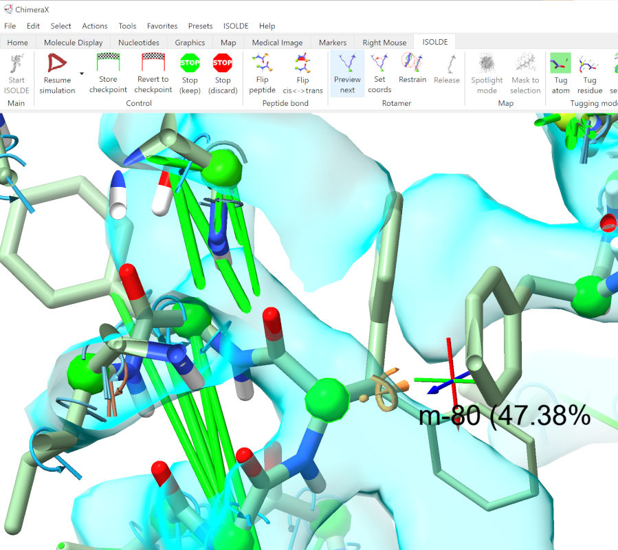
... then click the adjacent “Set coords” button. Do the same for the second PHE, then resume the simulation.
That should have resolved most of the issues with the helix itself, but the turn leading into the beta-hairpin is still in trouble, with restraints fighting against the density. The good news is that the density here is excellent - take a little time using the tools you’ve just learned to fix things up here. When you’re satisfied, stop the simulation.
NOTE: from this point forward things get a bit more challenging. One of the frustrations in structural biology is that we tend to spend very little time working on the beautiful high-resolution regions, and instead spend most of our time wrestling with the ugliest, noisiest parts of the map. Frustrating, but oh-so-satisfying when you find the right answer.
Time to take stock. Select the whole model:
... and expand the map to cover it, either using the “Mask to selection” button on ISOLDE’s ribbon menu, or the command:
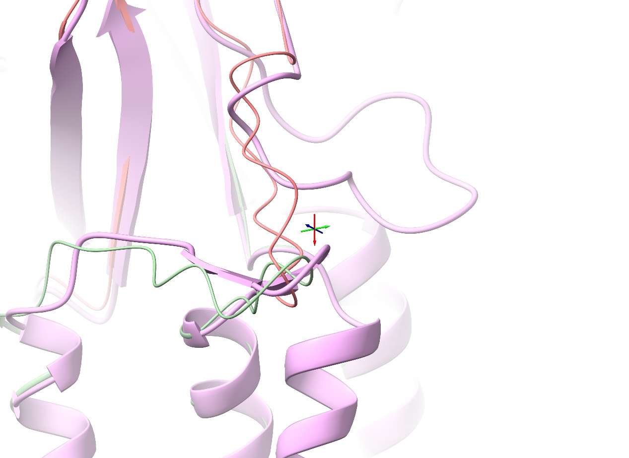
Take a look around and you’ll see that the overall fit of Wntless is looking pretty good (although there remains clear need for lots of local tidying - but it’s best to leave that until the really big issues are dealt with). The main body of Wnt3a, on the other hand, still seems to be well out of step with the density:
The problem here is that AlphaFold has predicted this contact as far more “intimate” that it actually is, and looking at the PAE matrix, it has done so with rather high confidence:
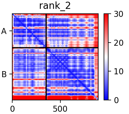
... leading to strong distance restraints holding it here. At this point I feel compelled to defend AlphaFold once again: while this prediction is not perfect, I cannot overstate how staggeringly good it is compared to everything that came before. Anyway, let’s see what we can do about that. The simplest approach is to simply release all restraints holding the two chains together, and that seems quite sensible in this case: the “good” parts of the interface are very close to their density and so should be fine without restraints, and the “bad” parts are… well, bad. Still, it’s best to do this in the context of a running simulation, since that allows us to revert if things go wrong (releasing restraints outside of a running simulation is currently an irreversible step).
Then,
isolde release distances /B to /C
... or equivalently:
This “to” option, allowing you to release only those restraints connecting one selection to another, is currently only available via commands.
Give it a minute or two, and it should settle much more comfortably into the density. Once you’re happy, stop the simulation:
... and bring up the reference model to take stock of how far things have shifted since we started:
Let’s zoom in on one of the Wnt3a residues for a closer look:
view #1/B:186; show #2/B:186; dist #2/B:186@CB|#1/B:186@CB color black
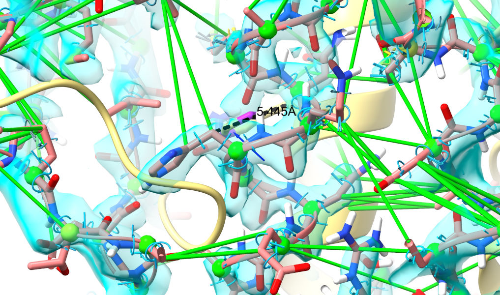
The main body of Wnt3a is now clearly in density, having shifted around 3-6 Angstroms from its starting position. Looking at the whole chain (something that can currently only be easily done via the Python console, I’m afraid), the range of shifts of alpha carbons in Wnt3a is around 0.5-12 Angstroms - in other words, some of the most tightly interacting residues have barely moved at all!
Anyway, moving forward. Let’s clean up the display again:
We’re getting much closer now, but there are still a few really challenging spots (where the density is challenging but not intractable, and the predicted model is particularly wrong) to deal with. To help with these, we’re going to do two things:
(a) Introduce a second, blurred version of the map, to more clearly show overall connectivity in the noisy regions:
(b) Increase the strength of the map’s “pull” on the atoms, to more clearly bring out the sites where it is “fighting” the restraints. Do this with the “Non-crystallographic Map Settings” on ISOLDE’s General tab, increasing the weight of each map from 0.04 to 0.1:
Now, start a simulation encompassing the whole model, and let it settle briefly:
Once you’re ready, stop the simulation:
... switch to ISOLDE’s “Problem Zones” tab, and click the Update button.
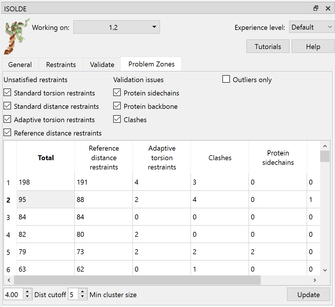
The aim of this widget is to look for clusters of “problems” (validation outliers, strained restraints) in 3D space, to help you find and tackle the biggest problems first. In this case the biggest cluster is actually a little boring - the bottom of the transmembrane domain, where the spacing between the helices was all a bit off in the starting geometry. Fixing that’s pretty trivial - just release the restraints between helices using the tools we’ve already seen (or, given the quality of the density, simply releasing all the restraints). Instead, click on the second row in the table.
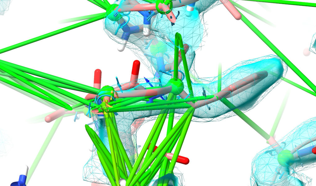
Yuck. That isn’t even close to correct (if you’ve really been paying attention, you’ll note that this is the same loop that was clashing horribly in the top-ranked model). Well, let’s roll up our sleeves and get to it. My general strategy when looking a a major rebuilding job like this is to follow the chain one direction to fine the “last good” residue (i.e. one making physical sense in good quality density), then extend a selection from there through the problem zone until I hit a good residue on the other end. Here, for example, Phe 161 looks very solid:
Select that (ctrl-click), then use the “Extend backward” button on ISOLDE’s Selection Tools panel to start growing the selection residue-by-residue towards the N-terminus.
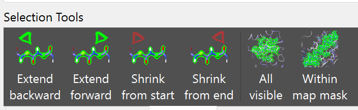
Do this until you hit another clearly-correct residue (ILE 135, if we discount the clearly-wrong rotamer).
Start a simulation:
The restraints in this region are clearly hopelessly wrong, so release them:
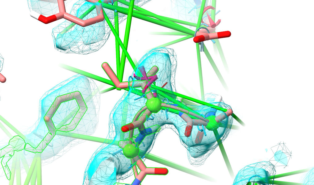
Dealing with this site is likely to take you quite a bit of trial and error - I’d recommend making aggressive use of the “checkpoint” buttons on ISOLDE’s ribbon menu to save the current state before trying a hypothesis, so you can revert if it doesn’t work out. The “Position Restraints” widget on ISOLDE’s Restraints tab can also be very useful, both for pinning well-placed residues to avoid accidentally displacing them, and to guide key atoms towards where you believe they belong. Before looking at the solution, spend some time playing around to see if you can figure it out. A few hints:
Look for the two closely-spaced tryptophan residues, and see if you can find similar-looking density;
One of the “arms” of the hairpin is much longer than the other. See if you can match this pattern in the density.
In this case it turns out the disulfide bonds are correct. If they weren’t, it would be possible to break and reform them via the ISOLDE/ Model Building/Disulphides menu.
The loop is very wrong - the kind of wrong that would almost certainly never be fixed by a straightforward “dumb” (unguided) simulation. You might find it easier to pull the tip of the loop out completely before rebuilding.
Once you do find it, the correct solution is fairly unmistakable.
Scroll down when you think you’re ready…
...
...
...
...
...
...
...
...
...
...
...
...
...
...
...
...
...
...
...
...
...
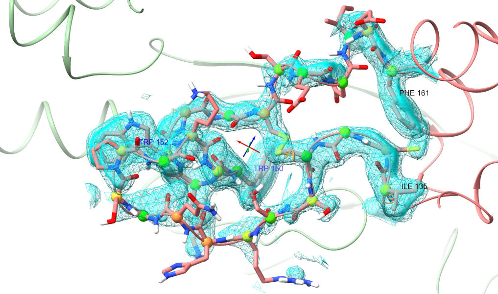
The result here is actually quite interesting. Clearly AlphaFold2 “knew” that a tryptophan belonged in the position occupied by TRP 150 - but it placed TRP152 there, and the knock-on effects from that led to the entire loop being twisted some 180 degrees from the experimental position.
If you’ve gotten this far, congratulations! Arguably the hardest part is now done - the overall fit is mostly good, and the worst mis-fit region has been rebuilt. At this stage, I would probably go ahead and release all the distance restraints using the “Remove all” button in the “Manage/Release Adaptive Restraints” widget, run a brief simulation to re-settle, then settle into the job of polishing the details. This is generally fairly straightforward in a map like this, and I find it quite relaxing. In brief:
... to go to the first residue in the model, and then repeat st to step forward residue-by-residue.
When you hit a problem, start a local simulation, release the necessary torsion restraints by selecting the residue(s) and doing rt
... and rebuilding as necessary. If you’re on a powerful workstation, running simulations in blocks of a few hundred residues (or even the whole model) at a time can speed things up markedly. Pro-tip: use the tools on the ChimeraX “Markers” tab to place markers at sites of interest or concern (e.g. blobs of unfilled density) so you can come back to them later. Actually placing ligands is beyond the scope of this particular tutorial, but if you really want to have a go for yourself, try the command “al {3-letter residue code}”.
Finally, a friendly reminder for when you want to apply what you’ve learned above to a new dataset: models coming straight from ISOLDE are currently not ready for deposition to the wwPDB. There are two main reasons for this:
The AMBER forcefield underlying ISOLDE (which attempts to replicate conformational energies from quantum mechanical simulations of model compounds) differs in various subtle ways from the libraries used for model validation (based on statistics derived from observations of high-resolution crystals). The validation report for a model settled in ISOLDE will give poor scores for bond length and angle RMSDs for this reason.
More importantly, ISOLDE currently makes no attempt to refine B-factors. Since B-factors encode our estimate of atom mobility relative to the bulk of the model, they are important in both cryo-EM and crystallography and should always be refined in a deposited model.
For the above reasons, before deposition you should always run a final refinement in your choice of package. If you’re using Phenix or REFMAC, the isolde write commands can be used to write suitable input files to your current working directory.