Introduction to crystallographic model rebuilding in ISOLDE
(NOTE: Most links on this page will only work correctly when the page is loaded in ChimeraX’s help viewer. You will also need to be connected to the Internet. Please close any open models before starting this tutorial.)
(The instructions in the tutorial below assume you are using a wired mouse with a scroll wheel doubling as the middle mouse button. While everything should also work well on touchpads in Windows and Linux, support for Apple’s multi-touch touchpad is a work in progress. Known issues with the latter are that clipping planes will not update when zooming, and recontouring of maps is not possible.)
Tutorial: Diagnosing and rebuilding errors in a 3Å crystal structure
Building models into low-resolution crystallographic density maps has traditionally been a difficult and often frustrating task. To illustrate why, let’s look at what happens to the density as resolution decreases. You can also use this as an opportunity to familiarise yourself with the controls.
Let’s start by looking at a small, high-resolution (1.1Å) model, 1a0m. The Clipper plugin allows you to fetch this directly from the wwPDB along with its structure factors using the ChimeraX command line:
open 1a0m structureFactors true
After running this command, check the ChimeraX log. You should see a warning message similar to that below:
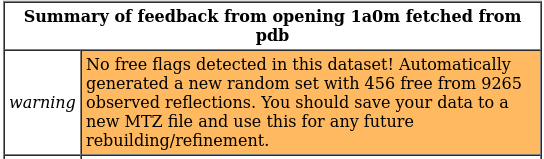
In crystallographic model building it is standard practice to leave a random selection of measured reflections (typically 5% or 2000 reflections, whichever is lower) as a guard against overfitting (see Brunger, 1992). While it is now standard practice for structure factors deposited to the wwPDB to include the free reflections used by the original modellers, this was not always the case. When no free flags are found a fresh set will be created for you - in such cases you should follow the advice in this warning and immediately save a fresh MTZ file incorporating these:
(OPTIONAL: personally I prefer to work with a white background. If you’re the same, you can change it using ChimeraX’s icons in the “Home” tab at top, or with the following command. You can also change it permanently using Favorites/Settings on the ChimeraX menu.)
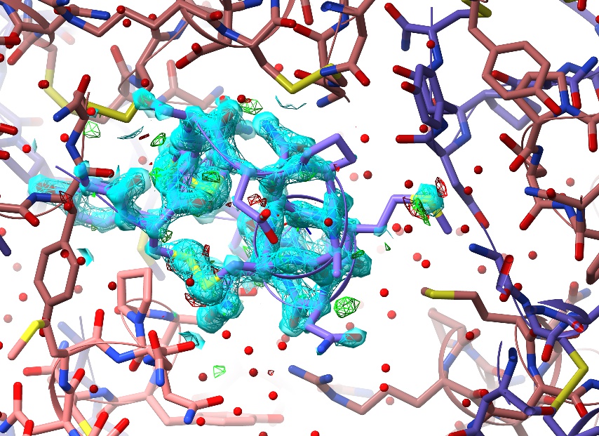
Now, zoom in by scrolling the mouse, and let’s go ahead and look at the model you just opened.
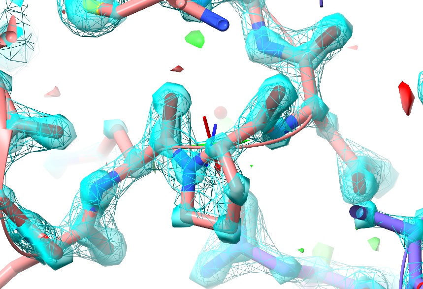
As you can see, at this resolution (almost) every non-hydrogen atom has its own distinct, clearly-differentiated “blob” of density - that is, the map shows you precisely where each individual atom belongs, and any errors in the model tend to be quite clear (and have equally clear solutions).
In this particular case, there are no real errors in the model - as one would hope given the resolution! While ultra-high-resolution models like this aren’t really what ISOLDE was designed for, this one makes for a nice “toy” to play with while learning the controls.
Getting around
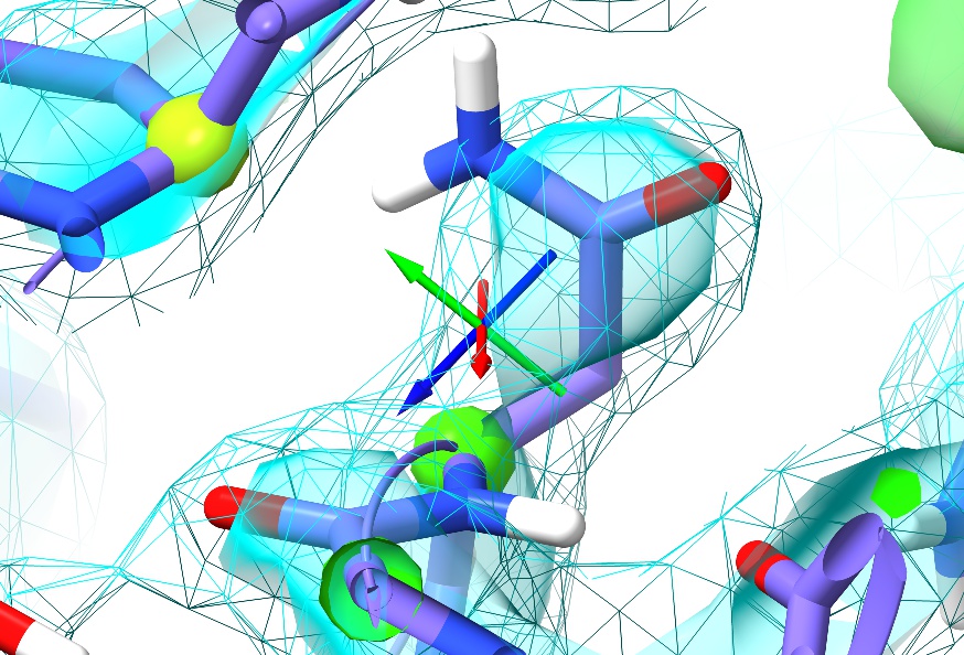
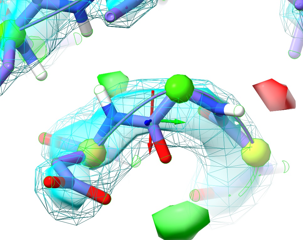
While zoomed in, you’ll notice a small set of axes displayed in the middle of the screen:
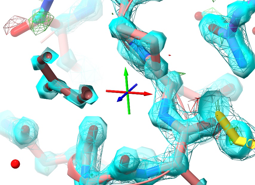
This is the pivot indicator marking the centre of rotation, and is useful as a reference point for certain tasks. The colours represent the three primary axes: red=x, green=y, blue=z.
When you zoom, the distance between the near and far clipping planes automatically grows and shrinks to provide depth cueing and reduce distracting clutter. If you need to adjust this, you can do so with shift-scroll.
Now, scroll out to a comfortable distance, and try panning. You have two options here: if you are using a wired mouse, just click and drag with the middle mouse button. For touchpad users without a middle-button equivalent, use shift-left-click-and-drag. To move the centre of rotation in the Z direction (that is, towards or away from you) use ctrl-middle-click-and-drag.
You’ll hopefully notice a few things:
Wherever you go, you’re surrounded by a sphere of density and displayed atoms. This is the default navigation mode in ISOLDE. The radius of the sphere can be controlled using the ISOLDE GUI (more on that in a bit) or using a command like clipper spotlight radius 15
Zoom out until you have a clear border all around the displayed atoms, then pan the mouse to the left. As you go, you’ll see a single cartoon start to stand out from the rest:
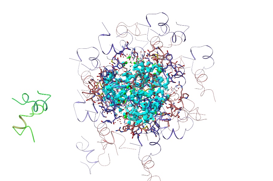
This is the actual model, which is always displayed in this mode - everything else is “ghost” drawings of the symmetry atoms (identifiable by their darker colour relative to the primary model). While you can’t interact directly with these, hovering over any symmetry atom will bring up a tool-tip giving its identity and symmetry operator, and double-clicking on one will re-centre your view on the equivalent “real” atom.
Adjusting your maps
When you load a model with structure factors, the Clipper plugin generates three maps: a standard 2mFo-DFc map; a second 2mFo-DFc map with either sharpening or smoothing applied depending on resolution (maps better than 2.5Å are smoothed, lower resolutions are sharpened); and a mFo-DFc map. The sharpest of the 2mFo-DFc maps is displayed as a transparent cyan surface, and the other as cyan wireframe. The sharper map gives the best detail in the well-resolved portions of the model, while the smoother one is better at revealing connectivity in poorly- resolved regions where sharp maps are often dominated by noise and difficult to interpret.
The difference map is shown as green and red wireframes for the positive and negative contours respectively.
On loading, contour levels are automatically chosen that are generally good for visualising the majority of the model - but you will of course need to adjust them from time to time. You can contour a given map using alt-scroll, and choose the map you wish to contour using ctrl-scroll.
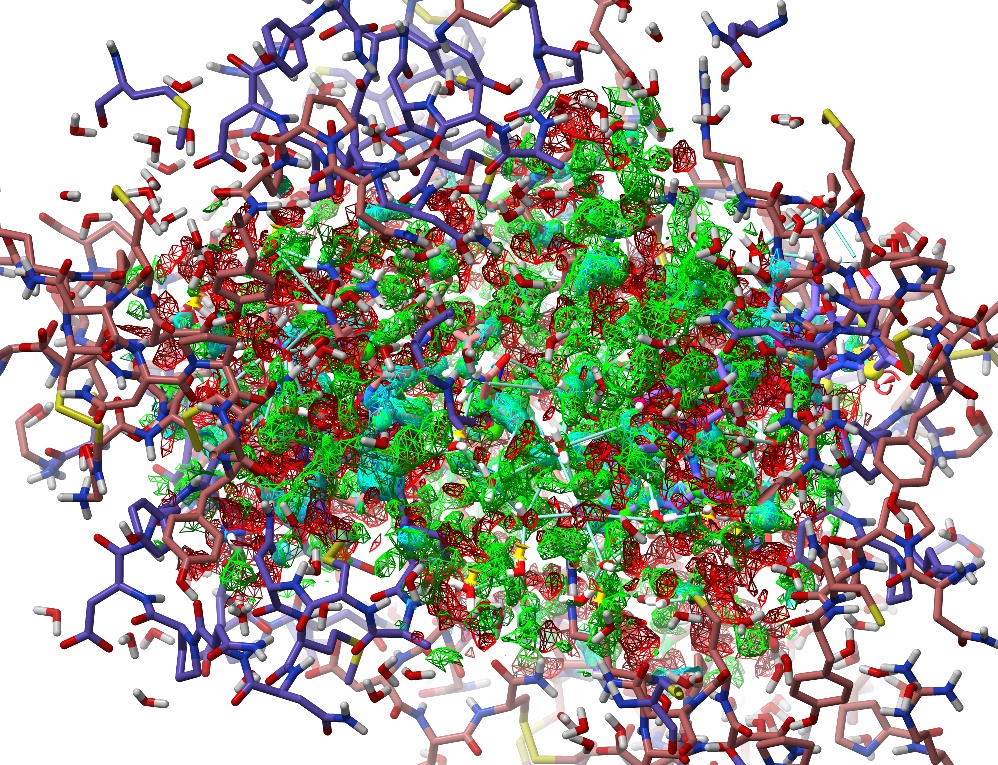
In many cases (particularly when working in low-resolution maps) you may wish to focus on some extended selection, where the default “sphere of density” view becomes impractical. You can expand and mask the map to cover any arbitrary selection using the clipper isolate command. For example:
… should give you something like this:
More specific selections can be specified using ChimeraX’s very powerful atomspec syntax.
You can further tweak the results using various optional arguments. To see the available options, use usage clipper isolate and check the Log window.
Once you’re done, go back to the scrolling-sphere mode using clipper spotlight.
Running your first simulation
Let’s go ahead and start ISOLDE. You can do this from the menu (Tools/General/ISOLDE) or by simply running the command isolde start.
A dialog box will pop up, notifying you that this model contains alternate conformers, and asking if you wish to remove them. In most of ISOLDE’s current use cases (where you may be making large changes to parts of the model) it is advisable to do so - currently there is no visible indicator of their presence, and ISOLDE will make no attempt to ensure that a given region remains structurally sensible relative to an alternate.
The next thing you may notice that all the C-alpha atoms in the model have suddenly turned into green spheres:
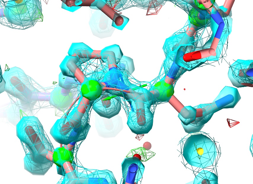
This is one example of ISOLDE’s real-time model validation, indicating each residue’s Ramachandran score (that is, the prior probability of the backbone “twist” around that residue). You can read more about this here.
If for any reason you wish to turn off display of any of ISOLDE’s validation or restraint markup, you can do so via the Models panel:
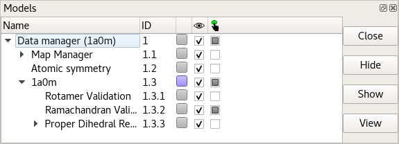
Just expand the drop-down list under the atomic model, and click the relevant checkbox under the eye icon. I would recommend against this in most cases, though: the information provided by the validation markup becomes very useful in guiding rebuilding, and there is nothing quite as frustrating as fighting against what turns out to be a restraint that you’ve hidden! If you wish, you can tell ISOLDE to show Ramachandran C-alpha markup for only non-favoured residues using the command:
… but personally, I prefer to keep them present. If you’re the same, put them back with:
Before we actually get things moving, it’s worth considering some of the strengths and pitfalls of molecular dynamics methods. Unlike minimisation using traditional Engh and Huber restraints, molecular dynamics attempts to realistically model all atomic interactions (including the van der Waals and electrostatic forces between non-bonded atoms) according to Newton’s laws of motion. In most ways this is extremely useful (as we will see), but the results can be problematic when it comes to very small ligands such as water molecules and monoatomic ions. In the absence of any explicit bonds to their neighbours, they can be prone to “wandering”. For this reason, ISOLDE provides a command allowing you to add explicit restraints to all small ligands in the model:
(NOTE: Validation and restraint markups are only drawn for real atoms, not their symmetry ghosts.)
By default, polar ligand atoms will receive distance restraints (represented by a cyan bar) to all other polar atoms within 4Å, and ligand residues with fewer than four distance restraints will be supplemented with position restraints (represented by a yellow pin). Note that these restraints are defined by the starting geometry (that is, they make no attempt to impose ideal geometry on the model), but are soft enough to allow substantial relaxation. Individual restraints can also be added, adjusted or removed using tools on ISOLDE’s “Rebuild” tab.
There is one more task we need to do before starting our first simulation: adding hydrogens. Like most molecular dynamics methods, ISOLDE requires residues to be chemically complete (with a few exceptions: “bare” N- and C-termini and sidechain truncations are permitted). ChimeraX’s AddH command typically does a great job of adding hydrogens. Just run:
By default, non-polar atoms are hidden, since these generally aren’t very interesting and tend to clutter up what is already quite a complex scene. If you really want to show them at any time, you can use:
... and hide them again with:
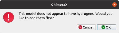
If you forget to add hydrogens before attempting to run a simulation, it’s not the end of the world. ISOLDE will bring up an error dialog like this:
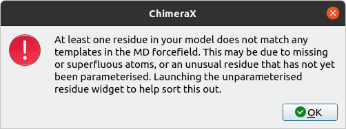
... and then, after clicking OK:
If you receive this error after adding hydrogens, stop and carefully inspect the offending residue with the aid of the Unparameterised Residues widget. Let’s force the issue, by deliberately deleting the hydrogens from a single residue:
Go to ISOLDE’s Validate tab, click the “Unparameterised Residues” button to expand the widget, and click “Update” at the bottom right. Click on the entry that appears in the top table. The result should look something like this:
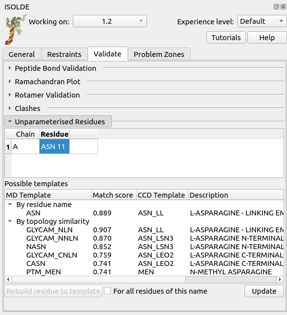
Here, the top table lists the problematic residues, while the bottom table lists all the MD templates ISOLDE thinks might match the currently-selected residue either due to name or to similar topology. In this case, the correct match is of course “ASN” - click that, then click “Rebuild residue to template” to fix the problem.
If there are no entries in the Possible Templates table, or no entries make sense to you, then it is likely that you are working with a new chemical species that ISOLDE doesn’t know about. In this case, all is not necessarily lost - if your problem ligand is (a) not covalently bound to anything else, and (b) made up only of the elements C, H, N, O, S, P, F, Cl, Br, and/or I, then you should be able to parameterise it using the “Residue Paramterisation” tool on ISOLDE’s General tab. We won’t talk further about that here, other than to say that when using this tool it is up to you to make sure the ligand is chemically correct first (all hydrogens present and in the right places, paying particular attention to protonation states of acidic and basic groups).
If you have a ligand or residue in your model which doesn’t fit the above description, then I’m afraid that handling it is currently outside the scope of ISOLDE’s capabilities. That shouldn’t necessarily stop you, though - this is one of the scenarios the isolde ignore command was made for, allowing you to exclude some portions of your model from simulations.
Anyway, in this case the simple addh command “just works” - so let’s go ahead and get the simulation moving. First, select the whole model:
... and either click ISOLDE’s blue “play” button (at the left of ISOLDE’s ribbon menu at the top of the ChimeraX screen) or use the command:
(NOTE: you do not HAVE to select the entire model to start a simulation in ISOLDE. As long as you have at least one atom selected, it will create a simulation with sufficient scope to encompass your region of interest surrounded by a soft “buffer zone” giving it freedom to work. In large models you should expect to spend most of your time in such “mini-simulations”, but - particularly at low resolutions - you should always run at least one “whole model” simulation to give any clashes and other very-high-energy states a chance to relax.)
After a few seconds, you should see your atoms start jiggling and the maps begin to regularly update. When working with crystallographic structure factors in ISOLDE, every change to the atomic coordinates, B-factors or occupancies triggers an automatic recalculation of structure factors, maps and R-factors. A running summary of the current R-factors is provided in the status bar at bottom right.
Interacting with the model
Now, try tugging on an atom using the right mouse button.
(NOTE: Non-polar hydrogens are not tuggable in ISOLDE. Polar hydrogens may be tugged, but in order to avoid instability the applied force will be much weaker than that applied to heavy atoms. While tugging on a hydrogen can be useful for adjusting the H-bonding of a hydroxyl group or water (for example), to make any larger changes you should choose a heavier atom to pull.)
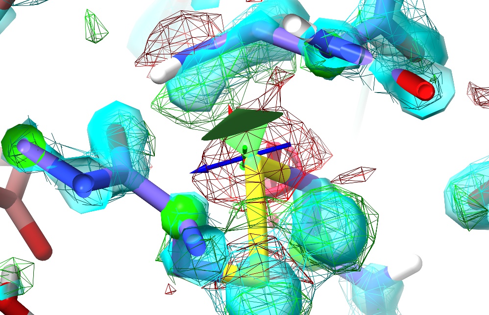
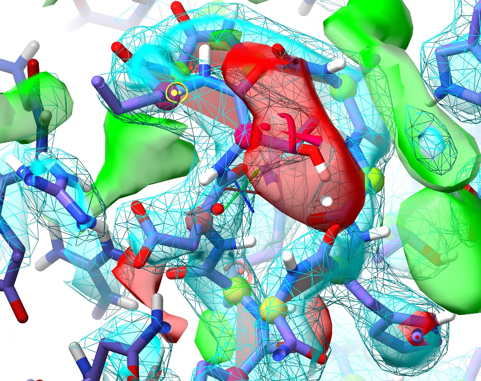
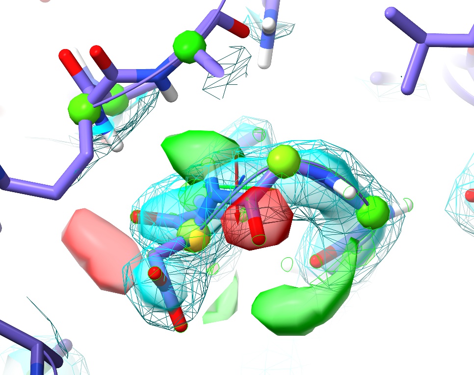
This should result in something like the above. There are a few things to note here:
The change in the maps (the large red blob around the sulphur atom, and the green blob where it used to be) is clearly telling you this is wrong (quite apart from the R-factors, which in this case have spiked from about 0.19 to around 0.26);
Tugging on the sulphur has had a knock-on effect on the adjacent Asn sidechain (top) - to re-iterate, in ISOLDE, all atoms feel each other.
You might wonder how the changes you see in the map affect the forces felt by the model. In short: every time the instantaneous R-work drops below the previous best value seen in the current simulation, the corresponding map is automatically used to update the fitting potential.
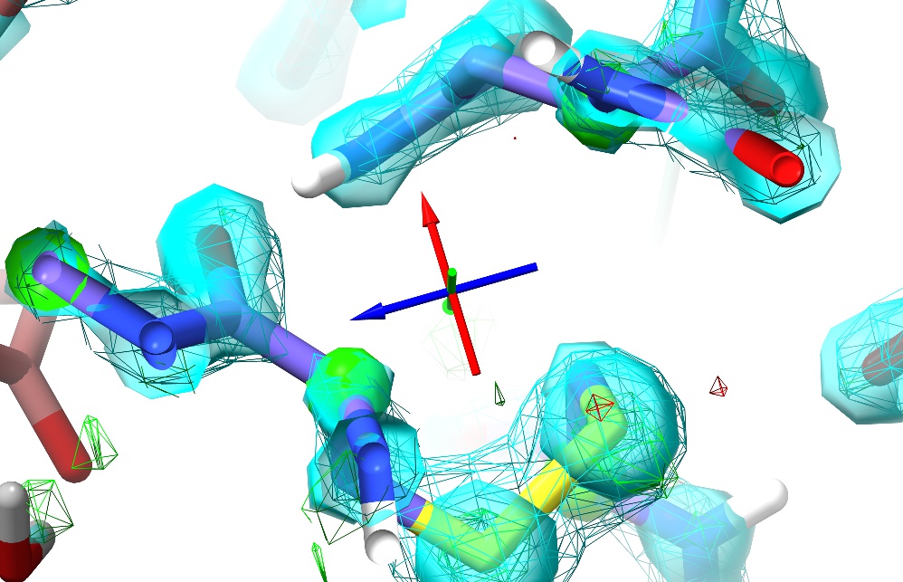
Unless you’ve done something particularly drastic, upon releasing the tugging force the model should snap back into place. In my case, here’s the model ~5 seconds later, with Rwork/Rfree back at 0.185/0.194:
The right mouse button is automatically mapped to this “tug single atom” mode every time a simulation is started. At the right of ISOLDE’s ribbon menu you will find three buttons allowing you to switch between this and “tug residue” or “tug selection”. These modes are primarily useful at much lower resolutions than this model.
General model controls
You may have noticed that ISOLDE’s blue play button has changed into a red pause symbol. Go ahead and click this to pause the simulation while we explore some of the other available controls.
First, go to ISOLDE’s General tab and click the “Dynamic Crystallographic Map Settings” button to expand that widget:
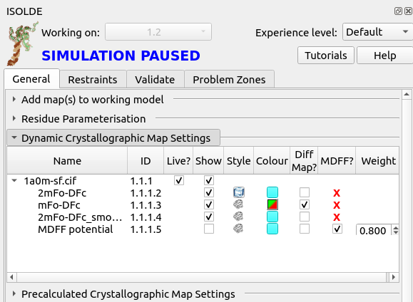
This gives you a listing of all “dynamic” maps (that is, those that are actively recalculated from the experimental reflection data) associated with the model, along with tools to adjust their behaviour. To get more information about each column, hover your mouse over the column title to bring up a brief tooltip.
Notice at the bottom, the map called “MDFF potential”. This defines the potential actually used for fitting in simulations, and is hidden by default. If you were to show it, it would actually look very similar to the displayed 2mFo-DFc maps, but there is one crucial difference: this map does not include contributions from the free reflections. That is very important, and is the reason why setting the other maps as MDFF potentials is not permitted - including the free reflections in the fitting potential would invalidate Rfree as a safeguard against overfitting.
On the far right of the MDFF potential line, you’ll see a number under the heading “Weight”. As the name suggests, this defines how strongly the potential pulls on atoms. When loading a new map, ISOLDE automatically chooses a suitable weighting based on the steepness of the gradients in the voxels immediately around the model atoms. The chosen weighting is usually quite sensible, but you may find you want to adjust it at times. This is where you can do that. Click the play button to get the model moving again, then change the weight to 0.1 and press return. You should see an immediate change in the model’s behaviour: the atoms will move much more “loosely”, more red and green will appear in the difference map, and the R-factors should increase to 0.24-0.26.
Injection of random positional error like this is one valid way to reduce the incidence of model bias that may arise due to the fact that we are not using the original free set. Note that since the fitting potential in a running simulation is only updated when the R-work drops to a new low, in this case you’ll have to stop the current simulation for the changes to take effect. Clicking the green “STOP” button at bottom right will stop the simulation and save the instantaneous coordinates. Now, set the weight back to 0.8, select the model and start a fresh simulation. You should see the R-factors quickly drop back to the vicinity of 0.19-0.21. Now, drop the temperature to zero using the slider near the bottom of the General tab. Wait for the R-factors to settle to constant values, and hit the green STOP button.
You may choose to continue with the temperature set to zero if you like, but personally I always prefer to have at least a little thermal motion happening - if for no other reason that it makes it easy to tell at a glance when a simulation is actually running! I’d suggest setting the temperature to 20-30K before continuing.
Now, let’s explore the other simulation control buttons. To the right of the play/pause button you’ll see two buttons with a green and red chequered flag respectively. These are the “checkpoint” controls. Clicking the green flag will save an instantaneous snapshot of the model as it is right now: not just the atomic positions, but all currently-active restraints. Go ahead and click it. Now, do something horrible to your model - just grab an atom and pull as hard as you can. You should see the map explode into a kaleidoscope of red and green, and the R-factors shoot up into the 0.4-0.6 range:
Whoops.
Click the red chequered flag to put everything back as it was. This is designed for the not-uncommon situation where the solution to a particular problem isn’t clear, allowing you to try out various hypotheses without the risk of permanent damage to the model.
To the right of the chequered flag you’ll find two different “STOP” buttons. The green one you’ve already used - it stops the simulation and keeps the current state. The red one discards the simulation entirely, returning the model to the state it was in at the moment the play button was pressed.
Rebuilding
While 1a0m is a useful model for learning to find your way around in ISOLDE, being very high-resolution and close to error-free means there is not really anything much to rebuild. So, let’s close it and move on to a more real-world task. Make sure you stop you simulation if you haven’t already:
… then close the model:
The model we’ll be looking at now is 3io0, a 3Å model of a small bacterial shell protein. This is discussed in more detail (including a video covering the whole rebuilding process) as a case study on the ISOLDE website.
To load these coordinates you could use “open 3io0 structureFactors true” as we did for 1a0m, but ISOLDE also keeps a locally cached version with hydrogens already added and an extraneous water molecule removed. To load it, click here.
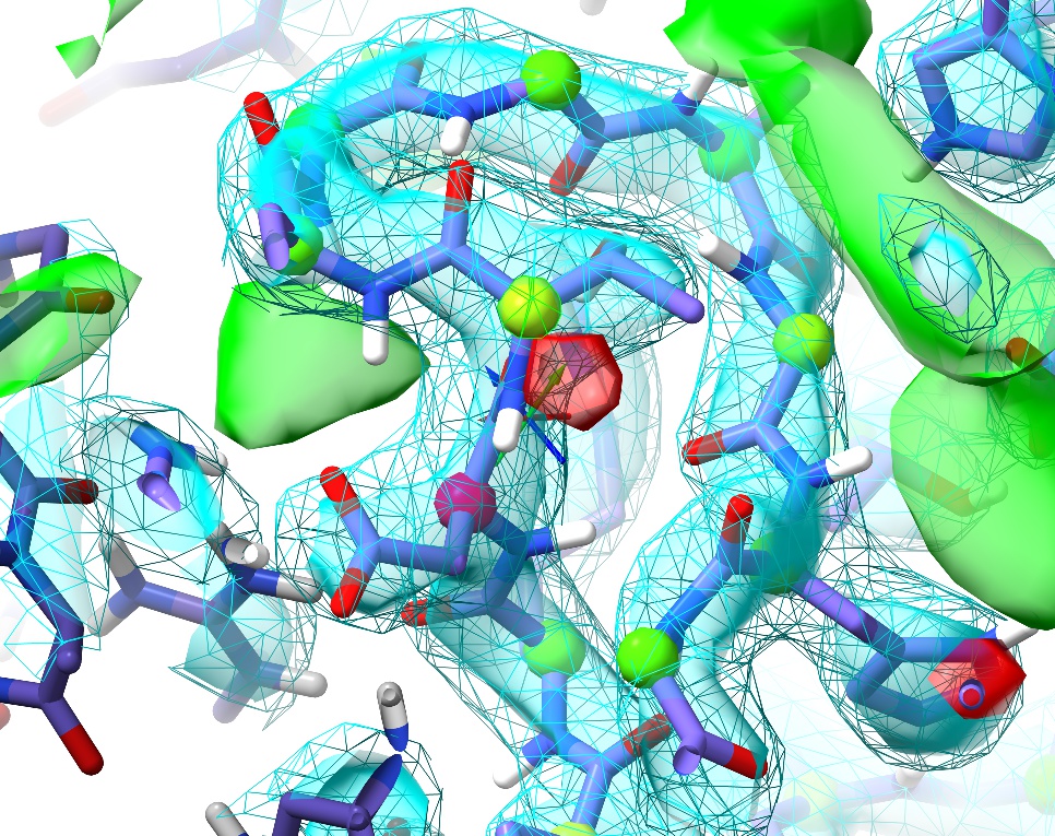
First, just have a browse around and compare the general appearance of the density to what you saw in 1a0m. For example, look at residue ASN187:
For the sake of comparison, here’s an asparagine in a similar environment in 1a0m (residue A9):

In the high-resolution model, not only is every non-hydrogen atom clearly resolved but the density even clearly shows the larger atomic radius of the oxygen compared to the nitrogen. In 3Å density, on the other hand, this detail is lost: the whole sidechain is reduced to an essentially featureless blob. The challenge such density poses given traditional restraint schemes is immense: with only weak guidance from the density itself and none from the non-bonded interactions with surroundings, finding the correct conformation out of all the possible incorrect conformations is, quite simply, hard. It is not surprising then that models of this resolution have historically been quite error-prone, and this one is no exception. In fact, a close look at Asn187 in context with its surroundings suggests it has been built backwards (with the oxygen occupying the space of the nitrogen and vice versa - look at the interactions with the peptide bond of Thr303 and the sidechain of Gln199 to see why).
Anyway, now is a good time to have a look at ISOLDE’s “Validate” tab. First, open up the Ramachandran plot, choose ‘All’ on the Case(s) drop-down menu, and take a look.
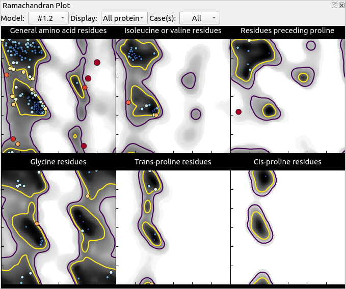
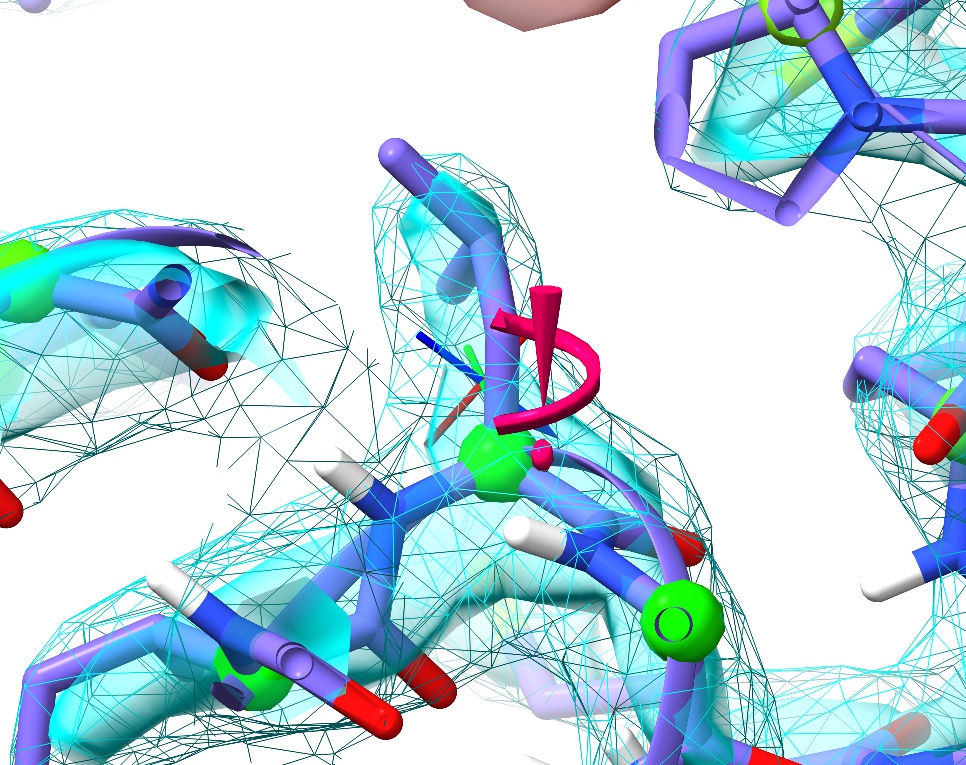
Mostly, this seems quite good, with only 3 outliers in the general case and one in “Residues preceding proline”. Hovering over any point in the plot will pop up a label with the residue ID, and clicking on it will centre the view on that residue. Find the outlier at Thr A84 (top right of the General plot) and click on it.
Hmm. Not only is this a Ramachandran outlier, but the red filled-in “cup” between adjacent alpha carbons highlights that it’s also a non-proline cis peptide bond. These are exceedingly rare in real life, and only occur in tightly-constrained, well-supported environments (which this isn’t). It will need to be fixed.
... But first, let’s go through the other validation tools. Close the Ramachandran plot, and show the “Peptide Bond Validation” widget. This provides a list with all questionable (cis or twisted) peptide bonds in the model. In this case we have seven non-proline cis bonds, two severely twisted peptide bonds, and one cis proline (unlike the non-proline case these are actually reasonably common at about 5% of proline residues). Click through the list and have a look - while the cis-pro looks happy, the rest appear unsupportable and will have to go.
Next, close the peptide bond widget and open the “Rotamer Validation” widget. Click on the first outlier in the list (Leu289).
Just like with the backbone Ramachandran conformation, sidechain rotamer outliers are marked up in real time. Problematic sidechains get the exclamation mark/spiral motif you see here. The size and colour of the marker will change depending on severity: a large, pink one like this denotes a severe outlier, whereas a marginal sidechain will show as a smaller yellow version.
Finally, close the rotamer widget and open the “Clashes” one. Once a simulation has started (provided that all atoms are mobile) the molecular dynamics forcefield ensures that clashes become effectively impossible - but the presence of any severe clashes in the starting coordinates should be a warning sign suggesting it would be best to run a simulation of the entire model at least once to resolve them before using more localised simulations to correct the errors we found above.
Let’s go ahead and do that:
If you’re on a machine with a powerful GPU, this should only take a few seconds, and a simulation running the entire model will likely be fast enough to work with, without the need to stop and restart with smaller selections. On slower hardware, just wait until you see the atoms start moving regularly - this indicates that the minimisation is complete and clashes are resolved. Once you hit the green stop button, it will be safe to start a simulation from any smaller selection. The remainder of the tutorial will assume you’re taking the latter approach - if you are lucky enough to be working with a fast GPU, just omit the stop/start steps.
Now, let’s take care of those cis bonds - since these are the most “unusual” conformations in the model, they seem like a sensible place to start. If you re-open the “Peptide bond geometry” widget and scroll to the bottom, you’ll see that the twisted peptides have taken care of themselves during the energy minimisation - ISOLDE assumes that any peptide bond twisted more than 30 degrees from cis should probably actually be trans, and restrains it as such.
Click on the top entry in the table. This will select the residue C-terminal to the offending bond and focus the display on it. Selecting a single amino acid like this also activates the “Peptide Bond” and “Rotamer” sections of ISOLDE’s ribbon menu. The “Flip cis<->trans” button up there can be used to correct the cis bond - but more conveniently, the table itself provides a “Flip” button for each cis bond it finds. Use whichever option you prefer. If you’re not currently running a simulation, ISOLDE will automatically start a small local one to do the job.
(NOTE: Most buttons in ISOLDE are only enabled under circumstances where it is sensible (and safe) to use them. The two different peptide flip buttons, for example, are only available when your selected atoms are from a single amino acid residue with a peptide bond N-terminal to it. Similarly, the rotamer selection buttons are only available when you have selected a non-truncated amino acid residue with at least one sidechain chi angle.)
Quite quickly, you should see something like this:
Voila! Not only is the cis peptide bond gone, but we’ve also corrected the Ramachandran outlier that was here into the bargain. On the other hand, now the sidechain is showing up as a severe rotamer outlier. Not to worry.
If you’ve deselected the residue, ctrl-click on an atom to select it again. Find and click the “Preview next” rotamer button in ISOLDE’s ribbon menu. This will create a preview of the most common rotamer for this residue overlaid on the existing coordinates, and show a lable with its name and statistical prevalence. Pressing it again will show the next most common rotamer, etc. - but in this case the first option looks good, with the hydroxyl pointing towards solvent, the methy pointing into the hydrophobic interface, and agreeing well with the density. The two buttons to the right allow you to either directly set the coordinates of the residue to match the preview, or add torsion restraints to force it towards the new conformation from its current state. The former option is fine in the majority of cases, but if there’s a chance the new conformation will clash with surrounding atoms it’s best to take the restraints option allowing it to more gently “push” its way into position. If you take the latter approach, the final (“Release”) button will, as the name suggests, release the torsion restraints.
Click the “Update” button in the Peptide Bond Validation widget, and click the new top entry. If you look around a little, you’ll see that there are actually six non-proline cis bonds in the vicinity, four of which are in tandem in one loop.
Let’s make a simulation selection that will cover all of them in one go. There are a few ways to go about this:
ctrl-shift-click on any atom to add it to the selection. Keep in mind that for each protein atom selected, when starting a simulation ISOLDE will automatically expand the selection to encompass its whole residue plus three residues forward and back along the chain.
Simply take advantage of ChimeraX’s selection promotion framework. If you have individual atoms selected, pressing the up arrow once will expand the selection to whole residues, and up again will further expand it to whole secondary structure elements (helices, strands or unstructured stretches). Pressing the down arrow will reverse the process. In this case, after clicking on the entry in the Peptide bond geometry table the offending residue is selected. Make sure the focus is on the main GUI window by left- clicking anywhere on the molecule, then press up once to select the whole loop with all six cis bonds.
Use the “Selection Tools” buttons at the bottom of the ISOLDE panel to grow/shrink selections by one residue at a time from their ends, or select all currently- visible atoms.
Once your selection is to your satisfaction, go ahead and click play to correct them. A handy way to remember which peptide bond will flip when you click the ribbon-menu button is to keep in mind that if you’ve selected an alpha carbon, the flip will be applied to the nitrogen directly bonded to it. If you accidentally flip one you didn’t mean to, it’s typically no big deal - just flip it right back.
Once these flips are done, You will also most likely find that you need to adjust the sidechains of Thr150 and Lys151 (although in some cases these correct themselves once the cis bonds are fixed). Also keep in mind that the peptide oxygen of Gly153 should end up pointing at the Arg148 sidechain - if this isn’t the case in your simulation, try using the “flip peptide bond” button (remember, it’s to the left of the cis<–>trans button).
(NOTE: this form of peptide bond flip can also be applied using the command “isolde pepflip sel”. Both “isolde pepflip” and “isolde cisflip” should be used with caution: while flipping every peptide bond in your model can certainly be entertaining, it’s not so much fun if you do so by accident.)
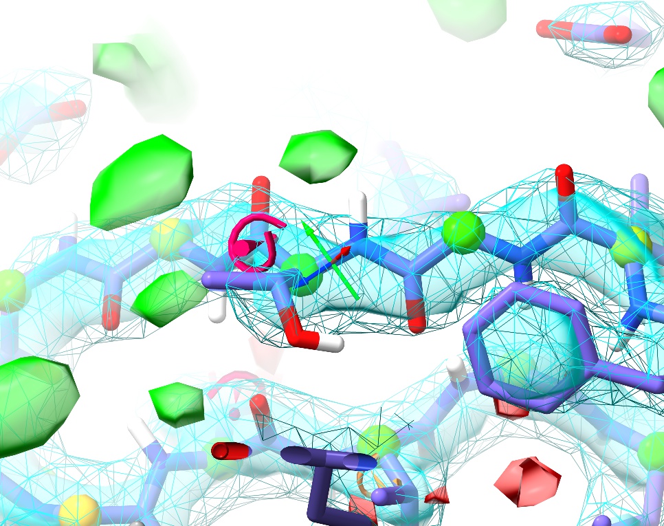
Once you’re done, the loop should look something like this:
The remaining Ramachandran outlier (pink C-alpha) at Asp149 appears to be a great example of the truism that not all Ramachandran outliers are wrong. In this case, the conformation not only fits well to the density, but makes perfect physical sense: the backbone twist is stabilised by charge interactions between the carbonyl oxygens and two nearby arginine residues (Arg148 in the same chain and Arg148 in the (y,z,x) symmetry copy), while the Asp149 sidechain is salt-bridged to Arg120 and further stabilised by two hydrogen bonds. This is what a Ramachandran outlier should look like: lots of energetically-favourable interactions overcoming the energy penalty associated with the unusual backbone twist.
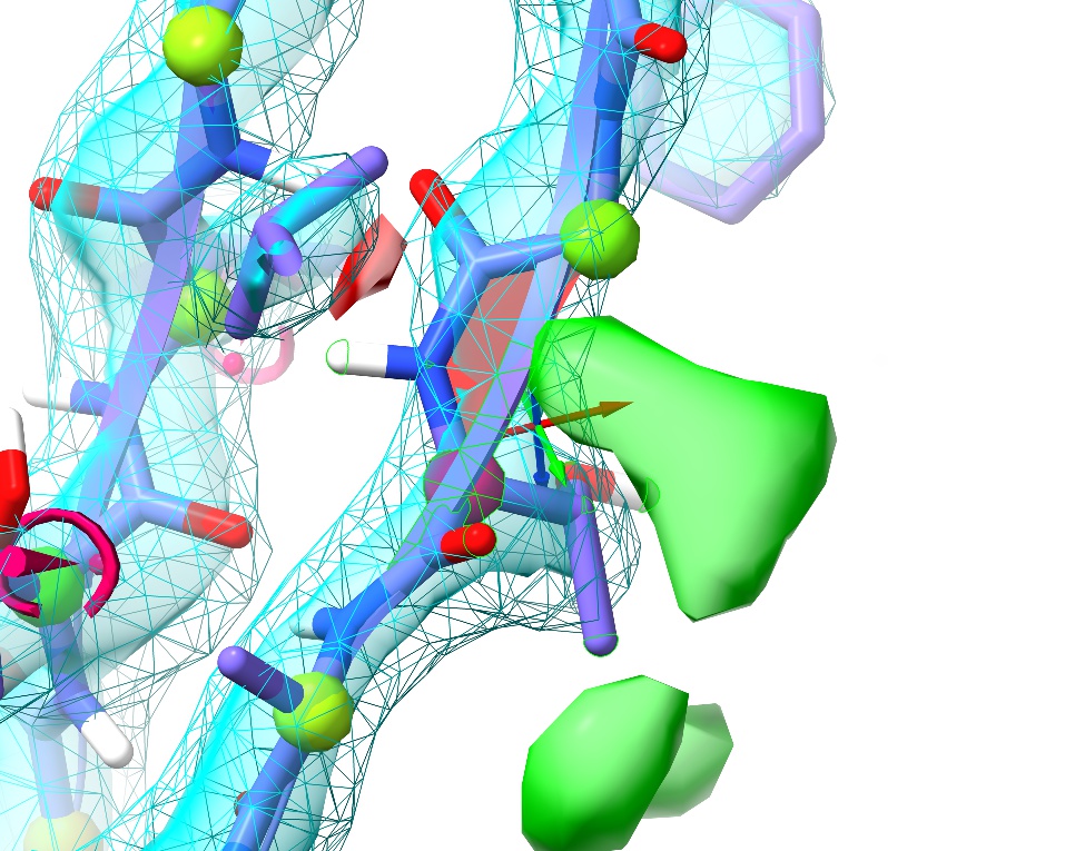
You may have noticed some positive (green) difference density in the channel to the right of this loop (when oriented like the image above), as well. This seems quite persistent throughout refinement, and may represent some low-occupancy ligand carried through during purification. At this resolution, though, it seems impossible to identify without further experimental knowledge.
Anyway, click the “Update” button in the Peptide Bond Validation widget to confirm that all the non-proline cis peptides are gone (if any still remain, fix them). Then, hide the “Peptide bond geometry” widget and we can move on.
From here, you could move on to working through the list of rotamer outliers in a similar manner, but it remains the case that in experimental model building, human eyes should see each residue in context with its density at least once. After all, it is entirely possible (and, in fact, quite common) for a model to find an incorrect conformation that is not an outlier by any standard metric but is nevertheless wrong.
The “isolde stepTo” command makes this easy, allowing you to systematically work through your model end-to-end. To make things even easier, let’s first run the command:
... and take a look at the log. This command defines a number of 2-4 character aliases for commands commonly used in ISOLDE. Once you’ve run it once, you can do:
... to jump to the first polymeric residue in your model, followed by simply
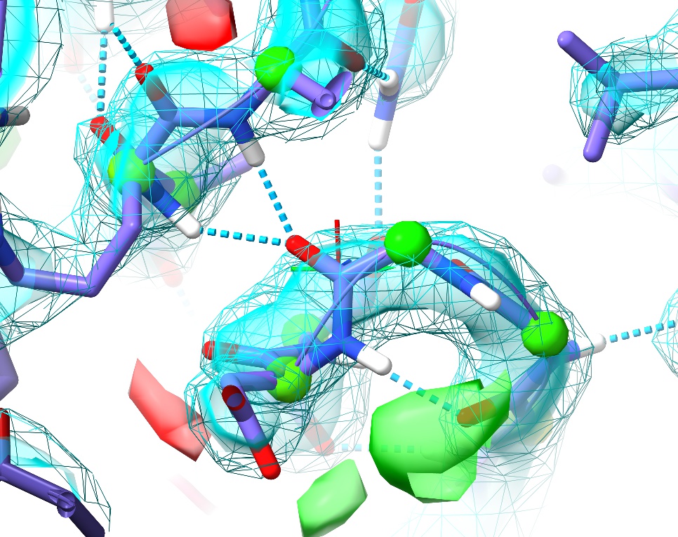
... to move to the next. Try this out for a while, stopping at any questionable residue (with yellow or pink validation markup, or poor fit to density) to see if you can improve it. One example I particularly want to highlight is at the first turn (between Gly87 and Asp88):
This is a perfect example of why it’s important to visually inspect the model. Here we have no sidechain nor Ramachandran outliers, yet the telltale paired red and green difference density blobs associated with the peptide oxygen and nitrogen say that this conformation is unquestionably wrong. Perhaps more concerning, in the original coordinates before energy minimisation in ISOLDE there was not even any sign of trouble in the difference density, and only a practised eye would notice the chemically-infeasible juxtaposition of the peptide hydrogen with those of Arg120 and Val121:
This highlights what I consider to be one of the strengths of the approach underlying ISOLDE: since the molecular dynamics forcefield is designed to closely replicate the physical reality of the molecule, it is much less likely to “fool you” in ways like this. Upon starting a simulation, the electrostatic repulsion between these positively charged groups pushes the incorrectly modelled peptide bond out of density, creating a clear red flag indicating something is wrong. In this case, the remedy is clear: a simple peptide flip creates two nice hydrogen bonds with the adjacent backbone (visualised here using ChimeraX’s H-bonds tool):
In addition, it places the backbone back in density (no more difference blobs), and as a bonus converts the slightly-marginal Ramachandran case at Asp88 into a favoured one. Don’t forget to hide the H-bonds display:
This covers most of the “workhorse” tools you’re likely to use for day-to-day work with models in medium-low resolution density with ISOLDE. Continue on through the rest of the model at your leisure. After some practice, I’ve found that I can improve this model to a MolProbity score below 1.0 in under 20 minutes (you can check for yourself using the MolProbity server or, if you have it installed, phenix.molprobity). If you want to refine and/or check your work using another package (recommended for any serious work: for a start, ISOLDE currently does not attempt to refine atomic B-factors), you can save your model and data at any time using the following commands.
save ~/Desktop/isolde_tutorial.pdb #1
save ~/Desktop/isolde_tutorial.mtz #1
If you have Phenix installed, you can prepare input files for it with my recommended refinement settings with:
isolde write phenixRef #1
This is not a clickable command in the tutorial, since that would write the resulting files into the tutorial directory rather than your current working directory. The command provides various extra options - do
... for more details.